Wasserstein-2 Optimal Transport (w2ot)
w2ot is JAX software by Brandon Amos
for estimating Wasserstein-2 optimal transport maps between
continuous measures in Euclidean space.
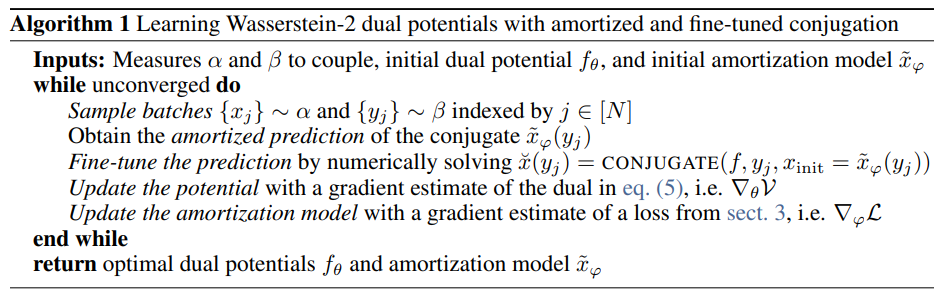
This is the official source code behind the paper
on amortizing convex conjugates for optimal transport,
which also unifies and implements the dual potential training from
Makkuva et al.,
Korotin et al. (Wasserstein-2 Generative Networks),
and Taghvaei and Jalali.
Getting started
Setup
pip install -r requirements.txt
python3 setup.py develop
Code structure
config # hydra config for the training setup
├── amortization
├── conjugate_solver
├── data # measures (or data) to couple
├── dual_trainer # main trainer object with model specifications
└── train.yaml # main entry point for running the code
scripts
├── analyze_2d_results.py # summarizes sweeps over 2d datasets
├── analyze_benchmark_results.py # summarizes sweeps over the W2 benchmarks
├── eval-conj-solver-benchmarks.py # evaluates the conj solver on the benchmarks
├── eval-conj-solver-lbfgs.py # ablates the LBFGS conj solvers
├── eval-conj-solver.py # evaluates the conj solver used for an experiment
├── prof-conj.py # profiles the conj solver
├── vis-2d-grid-warp.py # visualizes the grid warping by the OT map
└── vis-2d-transport.py # visualizes the transport map
w2ot # the main module
├── amortization.py # amortization choices
├── conjugate_solver.py # wrappers around conjugate solvers
├── data.py # connects all data into the same interface
├── dual_trainer.py # the main trainer for optimizing the W2 dual
├── external # Modified external code
├── models
│   ├── icnn.py # Input-convex neural network potential
│   ├── init_nn.py # An MLP amortization model
│   ├── potential_conv.py # A non-convex convolutional potential model
│   └── potential_nn.py # A non-convex MLP potential model
├── run_train.py # executable file for starting the training run
Running the 2d examples
A training run can be launched with w2ot/run_train.py, which specifies the dataset along with the choices for the models, amortization type, and conjugate solver. See the config directory for all of the available configuration options.
$ ./w2ot/run_train.py data=gauss8 dual_trainer=icnn amortization=regression conjugate_solver=lbfgs
This will write out the expermiental results to a local workspace
directory <exp_dir> that saves the latest and best models and logged metrics
about the progress.
scripts/vis-2d-transport.py produces additional visualizations about the learned transport potentials and the estimated optimal transport map:
$ ./scripts/vis-2d-transport.py <exp_dir>

scripts/vis-2d-grid-warp.py provides another visualization of how the transport warps a grid:
$ ./scripts/vis-2d-grid-warp.py <exp_dir>

Results in other 2d settings can be obtained similarly:
$ ./w2ot/run_train.py data=gauss_sq dual_trainer=icnn amortization=regression conjugate_solver=lbfgs
$ ./scripts/vis-2d-grid-warp.py <exp_dir>

Results on settings from Rout et al.
These are the circles, moons, s_curve, and swiss datasets.
Results on settings from Huang et al.
These are the maf_moon, rings, and moon_to_rings datasets.

Evaluating on the Wasserstein 2 benchmark
The software in this repository attains state-of-the-art performance on the Wasserstein-2 benchmark (code), which consists of two experimental settings that seek to recover known transport maps between measures.

Running a single instance
The configuration and code for these experiments can be specifed through hydra as before. To train an NN potential on the 256-dimensional HD benchmark with regression-based amortization and an LBFGS conjugate solver, run:
$ ./w2ot/run_train.py data=benchmark_hd dual_trainer=nn_hd_benchmark amortization=regression data.input_dim=256 conjugate_solver=lbfgs
A single run for the CelebA part of the benchmark can similarly be run with:
$ ./w2ot/run_train.py data=benchmark_images dual_trainer=image_benchmark data.which=Early amortization=regression conjugate_solver=lbfgs
Running the main sweep
All of the experimental results can be obtained by launching a sweep with hydra’s multirun option.
$ ./w2ot/run_train.py -m seed=$(seq -s, 10) data=benchmark_images dual_trainer=image_benchmark data.which=Early,Mid,Late amortization=objective,objective_finetune,regression,w2gn,w2gn_finetune
$ ./train.py -m seed=$(seq -s, 10) data=benchmark_hd dual_trainer=icnn_hd_benchmark,nn_hd_benchmark amortization=objective,objective_finetune,regression,w2gn,w2gn_finetune data.input_dim=2,4,8,16,32,64,128,256
The following code synthesizes the results from these runs and outputs the LaTeX source code for the tables that appear in the paper:
./analyze_benchmark_results.py <exp_root> # Output main tables.
Extending this software
I have written this code to make it easy to add new measures, dual training methods, and conjugate solvers.
Adding new measures and data
Add a new config entry to config/data pointing to the samplers for the measures, which you can add to w2ot/data.py.
Adding a new training method
If your new method is a variant of the dual potential-based approach, you may be able to add the right new config options and implementations to w2ot/dual_trainer.py. Otherwise, it may be simpler to copy this and create another trainer with a similar interface.
Adding a new conjugate solver
Add a new config entry to config/conjugate_solver pointing to your conjugate solver, which should follow the same interface as the ones in w2ot/conjugate_solver.py.
Licensing
Unless otherwise stated, the source code in this repository is licensed under the Apache 2.0 License. The code in w2ot/external contains modified external software from jax, jaxopt, Wasserstein2Benchmark, and ott that remain under the original license.


