JAX: Autograd and XLA
JAX is Autograd and XLA, brought together for high-performance machine learning research.
With its updated version of Autograd, JAX can automatically differentiate native Python and NumPy functions. It can differentiate through loops, branches, recursion, and closures, and it can take derivatives of derivatives of derivatives. It supports reverse-mode differentiation (a.k.a. backpropagation) as well as forward-mode differentiation, and the two can be composed arbitrarily to any order.
What’s new is that JAX uses XLA to compile and run your NumPy programs on GPUs and TPUs. Compilation happens under the hood by default, with library calls getting just-in-time compiled and executed. But JAX also lets you just-in-time compile your own Python functions into XLA-optimized kernels using a one-function API, jit. Compilation and automatic differentiation can be composed arbitrarily, so you can express sophisticated algorithms and get maximal performance without leaving Python.
This is a research project, not an official Google product. Expect bugs and sharp edges. Please help by trying it out, reporting bugs, and letting us know what you think!
import jax.numpy as np
from jax import grad, jit, vmap
from functools import partial

def predict(params, inputs):
  for W, b in params:
    outputs = np.dot(inputs, W) + b
    inputs = np.tanh(outputs)
  return outputs

def logprob_fun(params, inputs, targets):
  preds = predict(params, inputs)
  return np.sum((preds - targets)**2)

grad_fun = jit(grad(logprob_fun))  # compiled gradient evaluation function
perex_grads = jit(lambda params, inputs, targets:  # fast per-example gradients
                  vmap(partial(grad_fun, params), inputs, targets))
Quickstart: Colab in the Cloud
Jump right in using a notebook in your
browser
connected to a Google Cloud GPU.
Installation
JAX is written in pure Python, but it depends on XLA, which needs to be
compiled and installed as the jaxlib package. Use the following instructions
to build JAX from source or install a binary package with pip.
Building JAX from source
First, obtain the JAX source code:
git clone https://github.com/google/jax
cd jax
To build XLA with CUDA support, you can run
python build/build.py --enable_cuda
pip install -e build  # install jaxlib (includes XLA)
pip install -e .      # install jax (pure Python)
See python build/build.py --help for configuration options, including ways to
specify the paths to CUDA and CUDNN, which you must have installed. The build
also depends on NumPy, and a compiler toolchain corresponding to that of
Ubuntu 16.04 or newer.
To build XLA without CUDA GPU support (CPU only), drop the --enable_cuda:
python build/build.py
pip install -e build  # install jaxlib (includes XLA)
pip install -e .      # install jax
To upgrade to the latest version from GitHub, just run git pull from the JAX
repository root, and rebuild by running build.py if necessary. You shouldn't have
to reinstall because pip install -e sets up symbolic links from site-packages
into the repository.
pip installation
Installing XLA with prebuilt binaries via pip is still experimental,
especially with GPU support. Let us know on the issue
tracker if you run into any errors.
To install a CPU-only version, which might be useful for doing local
development on a laptop, you can run
pip install jax jaxlib # CPU-only version
If you want to install JAX with both CPU and GPU support, using existing CUDA
and CUDNN7 installations on your machine (for example, preinstalled on your
cloud VM), you can run
# install jaxlib
PYTHON_VERSION=py2  # alternatives: py2, py3
CUDA_VERSION=cuda92  # alternatives: cuda90, cuda92, cuda100
PLATFORM=linux_x86_64  # alternatives: linux_x86_64
pip install https://storage.googleapis.com/jax-wheels/$CUDA_VERSION/jaxlib-0.1-$PYTHON_VERSION-none-$PLATFORM.whl

pip install jax  # install jax
The library package name must correspond to the version of the existing CUDA
installation you want to use, with cuda100 for CUDA 10.0, cuda92 for CUDA
9.2, and cuda90 for CUDA 9.0. To find your CUDA and CUDNN versions, you can
run command like these, depending on your CUDNN install path:
nvcc --version
grep CUDNN_MAJOR -A 2 /usr/local/cuda/include/cudnn.h  # might need different path
A brief tour
In [1]: import jax.numpy as np

In [2]: from jax import random

In [3]: key = random.PRNGKey(0)

In [4]: x = random.normal(key, (5000, 5000))

In [5]: print(np.dot(x, x.T) / 2)  # fast!
[[  2.52727051e+03   8.15895557e+00  -8.53276134e-01 ...,  # ...

In [6]: print(np.dot(x, x.T) / 2)  # even faster!
[[  2.52727051e+03   8.15895557e+00  -8.53276134e-01 ...,  # ...
What’s happening behind-the-scenes is that JAX is using XLA to just-in-time
(JIT) compile and execute these individual operations on the GPU. First the
random.normal call is compiled and the array referred to by x is generated
on the GPU. Next, each function called on x (namely transpose, dot, and
divide) is individually JIT-compiled and executed, each keeping its results on
the device.
It’s only when a value needs to be printed, plotted, saved, or passed into a raw
NumPy function that a read-only copy of the value is brought back to the host as
an ndarray and cached. The second call to dot is faster because the
JIT-compiled code is cached and reused, saving the compilation time.
The fun really starts when you use grad for automatic differentiation and
jit to compile your own functions end-to-end. Here’s a more complete toy
example:
from jax import grad, jit
import jax.numpy as np

def sigmoid(x):
    return 0.5 * (np.tanh(x / 2.) + 1)

# Outputs probability of a label being true according to logistic model.
def logistic_predictions(weights, inputs):
    return sigmoid(np.dot(inputs, weights))

# Training loss is the negative log-likelihood of the training labels.
def loss(weights, inputs, targets):
    preds = logistic_predictions(weights, inputs)
    label_probs = preds * targets + (1 - preds) * (1 - targets)
    return -np.sum(np.log(label_probs))

# Build a toy dataset.
inputs = np.array([[0.52, 1.12,  0.77],
                   [0.88, -1.08, 0.15],
                   [0.52, 0.06, -1.30],
                   [0.74, -2.49, 1.39]])
targets = np.array([True, True, False, True])

# Define a compiled function that returns gradients of the training loss
training_gradient_fun = jit(grad(loss))

# Optimize weights using gradient descent.
weights = np.array([0.0, 0.0, 0.0])
print("Initial loss: {:0.2f}".format(loss(weights, inputs, targets)))
for i in range(100):
    weights -= 0.1 * training_gradient_fun(weights, inputs, targets)

print("Trained loss: {:0.2f}".format(loss(weights, inputs, targets)))
To see more, check out the quickstart
notebook,
a simple MNIST classifier
example
and the rest of the JAX
examples.
What's supported
If you’re using JAX just as an accelerator-backed NumPy, without using grad or
jit in your code, then in principle there are no constraints, though some
NumPy functions haven’t been implemented yet. Generally using np.dot(A, B) is
better than A.dot(B) because the former gives us more opportunities to run the
computation on the device. NumPy also does a lot of work to cast any array-like
function arguments to arrays, as in np.sum([x, y]), while jax.numpy
typically requires explicit casting of array arguments, like
np.sum(np.array([x, y])).
For automatic differentiation with grad, JAX has the same restrictions
as Autograd. Specifically, differentiation
works with indexing (x = A[i, j, :]) but not indexed assignment (A[i, j] = x) or indexed in-place updating (A[i] += b). You can use lists, tuples, and
dicts freely: jax doesn't even see them. Using np.dot(A, B) rather than
A.dot(B) is required for automatic differentiation when A is a raw ndarray.
For compiling your own functions with jit there are a few more requirements.
Because jit aims to specialize Python functions only on shapes and dtypes
during tracing, rather than on concrete values, Python control flow that depends
on concrete values won’t be able to execute and will instead raise an error. If
you want compiled control flow, use structured control flow primitives like
lax.cond and lax.while. Some indexing features, like slice-based indexing
A[i:i+5] for argument-dependent i, or boolean-based indexing A[bool_ind]
for argument-dependent bool_ind, produce abstract values of unknown shape and
are thus unsupported in jit functions.
In general, JAX is intended to be used with a functional style of Python
programming. Functions passed to transformations like grad and jit are
expected to be free of side-effects. You can write print statements for
debugging but they may only be executed once if they're under a jit decorator.
TLDR Do use
- Functional programming
- Many of NumPy’s
functions (help us add more!)- Some SciPy functions
- Indexing and slicing of arrays like
x = A[[5, 1, 7], :, 2:4]- Explicit array creation from lists like
A = np.array([x, y])Don’t use
- Assignment into arrays like
A[0, 0] = x- Implicit casting to arrays like
np.sum([x, y])(usenp.sum(np.array([x, y])instead)A.dot(B)method syntax for functions of more than one argument (use
np.dot(A, B)instead)- Side-effects like mutation of arguments or mutation of global variables
- The
outargument of NumPy functionsFor jit functions, also don’t use
- Control flow based on dynamic values
if x > 0: .... Control flow based
on shapes is fine:if x.shape[0] > 2: ...andfor subarr in array.- Slicing
A[i:i+5]for dynamic indexi(uselax.dynamic_sliceinstead)
or boolean indexingA[bool_ind]for traced valuesbool_ind.
You should get loud errors if your code violates any of these.
Transformations
At its core, JAX is an extensible system for transforming numerical functions.
We currently expose three important transformations: grad, jit, and vmap.
Automatic differentiation with grad
JAX has roughly the same API as Autograd.
The most popular function is grad for reverse-mode gradients:
from jax import grad
import jax.numpy as np

def tanh(x):  # Define a function
  y = np.exp(-2.0 * x)
  return (1.0 - y) / (1.0 + y)

grad_tanh = grad(tanh)  # Obtain its gradient function
print(grad_tanh(1.0))   # Evaluate it at x = 1.0
# prints 0.41997434161402603
You can differentiate to any order with grad.
For more advanced autodiff, you can use jax.vjp for reverse-mode
vector-Jacobian products and jax.jvp for forward-mode Jacobian-vector
products. The two can be composed arbitrarily with one another, and with other
JAX transformations. Here's one way to compose
those to make a function that efficiently computes full Hessian matrices:
from jax import jit, jacfwd, jacrev
def hessian(fun):
  return jit(jacfwd(jacrev(fun)))
As with Autograd, you're free to use differentiation with Python control
structures:
def abs_val(x):
  if x > 0:
    return x
  else:
    return -x

abs_val_grad = grad(abs_val)
print(abs_val_grad(1.0))   # prints 1.0
print(abs_val_grad(-1.0))  # prints -1.0 (abs_val is re-evaluated)
Compilation with jit
You can use XLA to compile your functions end-to-end with jit, used either as
an @jit decorator or as a higher-order function.
import jax.numpy as np
from jax import jit

def slow_f(x):
  # Element-wise ops see a large benefit from fusion
  return x * x + x * 2.0

x = np.ones((5000, 5000))
fast_f = jit(slow_f)
%timeit -n10 -r3 fast_f(x)  # ~ 4.5 ms / loop on Titan X
%timeit -n10 -r3 slow_f(x)  # ~ 14.5 ms / loop (also on GPU via JAX)
You can mix jit and grad and any other JAX transformation however you like.
Auto-vectorization with vmap
vmap is the vectorizing map.
It has the familiar semantics of mapping a function along array axes, but
instead of keeping the loop on the outside, it pushes the loop down into a
function’s primitive operations for better performance.
Using vmap can save you from having to carry around batch dimensions in your
code. For example, consider this simple unbatched neural network prediction
function:
def predict(params, input_vec):
  assert input_vec.ndim == 1
  for W, b in params:
    output_vec = np.dot(W, input_vec) + b  # `input_vec` on the right-hand side!
    input_vec = np.tanh(output_vec)
  return output_vec
We often instead write np.dot(inputs, W) to allow for a batch dimension on the
left side of inputs, but we’ve written this particular prediction function to
apply only to single input vectors. If we wanted to apply this function to a
batch of inputs at once, semantically we could just write
from functools import partial
predictions = np.stack(list(map(partial(predict, params), input_batch)))
But pushing one example through the network at a time would be slow! It’s better
to vectorize the computation, so that at every layer we’re doing matrix-matrix
multiplies rather than matrix-vector multiplies.
The vmap function does that transformation for us. That is, if we write
from jax import vmap
predictions = vmap(partial(predict, params), input_batch)
then the vmap function will push the outer loop inside the function, and our
machine will end up executing matrix-matrix multiplications exactly as if we’d
done the batching by hand.
It’s easy enough to manually batch a simple neural network without vmap, but
in other cases manual vectorization can be impractical or impossible. Take the
problem of efficiently computing per-example gradients: that is, for a fixed set
of parameters, we want to compute the gradient of our loss function evaluated
separately at each example in a batch. With vmap, it’s easy:
per_example_gradients = vmap(partial(grad(loss), params), inputs, targets)
Of course, vmap can be arbitrarily composed with jit, grad, and any other
JAX transformation! We use vmap with both forward- and reverse-mode automatic
differentiation for fast Jacobian and Hessian matrix calculations in
jax.jacfwd, jax.jacrev, and jax.hessian.
Random numbers are different
JAX needs a functional pseudo-random number generator (PRNG) system to provide
reproducible results invariant to compilation boundaries and backends, while
also maximizing performance by enabling vectorized generation and
parallelization across random calls. The numpy.random library doesn’t have
those properties. The jax.random library meets those needs: it’s functionally
pure, but it doesn’t require you to pass stateful random objects back out of
every function.
The jax.random library uses
count-based PRNGs
and a functional array-oriented
splitting model.
To generate random values, you call a function like jax.random.normal and give
it a PRNG key:
import jax.random as random

key = random.PRNGKey(0)
print(random.normal(key, shape=(3,)))  # [ 1.81608593 -0.48262325  0.33988902]
If we make the same call again with the same key, we get the same values:
print(random.normal(key, shape=(3,))) # [ 1.81608593 -0.48262325 0.33988902]
The key never gets updated. So how do we get fresh random values? We use
jax.random.split to create new keys from existing ones. A common pattern is to
split off a new key for every function call that needs random values:
key = random.PRNGKey(0)

key, subkey = random.split(key)
print(random.normal(subkey, shape=(3,)))  # [ 1.1378783  -1.22095478 -0.59153646]

key, subkey = random.split(key)
print(random.normal(subkey, shape=(3,)))  # [-0.06607265  0.16676566  1.17800343]
By splitting the PRNG key, not only do we avoid having to thread random states
back out of every function call, but also we can generate multiple random arrays
in parallel because we can avoid unnecessary sequential dependencies.
There's a gotcha here, which is that it's easy to unintentionally reuse a key
without splitting. We intend to add a check for this (a sort of dynamic linear
typing) but for now it's something to be careful about.
Mini-libraries
JAX provides some small, experimental libraries for machine learning. These
libraries are in part about providing tools and in part about serving as
examples for how to build such libraries using JAX. Each one is only a few
hundred lines of code, so take a look inside and adapt them as you need!
Neural-net building with Stax
Stax is a functional neural network building library. The basic idea is that
a single layer or an entire network can be modeled as an (init_fun, apply_fun)
pair. The init_fun is used to initialize network parameters and the
apply_fun takes parameters and inputs to produce outputs. There are
constructor functions for common basic pairs, like Conv and Relu, and these
pairs can be composed in series using stax.serial or in parallel using
stax.parallel.
Here’s an example:
from jax.experimental import stax
from jax.experimental.stax import Conv
from jax.experimental.stax import Dense
from jax.experimental.stax import MaxPool
from jax.experimental.stax import Relu
from jax.experimental.stax import LogSoftmax

# Set up network initialization and evaluation functions
net_init, net_apply = stax.serial(
    Conv(32, (3, 3), padding='SAME'), Relu,
    Conv(64, (3, 3), padding='SAME'), Relu,
    MaxPool((2, 2)), Flatten,
    Dense(128), Relu,
    Dense(10), SoftMax,
)

# Initialize parameters, not committing to a batch shape
in_shape = (-1, 28 * 28)
out_shape, net_params = net_init(in_shape)

# Apply network
predictions = net_apply(net_params, inputs)
First-order optimization with Minmax
Minmax is an optimization library focused on stochastic first-order
optimizers. Every optimizer is modeled as an (init_fun, update_fun) pair. The
init_fun is used to initialize the optimizer state, which could include things
like momentum variables, and the update_fun accepts a gradient and an
optimizer state to produce a new optimizer state. The parameters being optimized
can be ndarrays or arbitrarily-nested list/tuple/dict structures, so you can
store your parameters however you’d like.
Here’s an example, using jit to compile the whole update end-to-end:
from jax.experimental import minmax
from jax import jit

# Set up an optimizer
opt_init, opt_update = minmax.momentum(step_size=1e-3, mass=0.9)

# Define a compiled update step
@jit
def step(i, opt_state, batch):
  params = minmax.get_params(opt_state)
  g = grad(loss)(params, batch)
  return opt_update(i, g, opt_state)

# Optimize parameters in a loop
opt_state = opt_init(net_params)
for i in range(num_steps):
  opt_state = step(i, opt_state, next(data_generator))
net_params = minmax.get_params(opt_state)
How it works
Programming in machine learning is about expressing and transforming functions.
Transformations include automatic differentiation, compilation for accelerators,
and automatic batching. High-level languages like Python are great for
expressing functions, but usually all we can do with them is apply them. We lose
access to their internal structure which would let us perform transformations.
JAX is a tool for specializing and translating high-level Python+NumPy functions
into a representation that can be transformed and then lifted back into a Python
function.
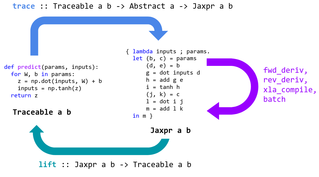
JAX specializes Python functions by tracing. Tracing a function means monitoring
all the basic operations that are applied to its input to produce its output,
and recording these operations and the data-flow between them in a directed
acyclic graph (DAG). To perform tracing, JAX wraps primitive operations, like
basic numerical kernels, so that when they’re called they add themselves to a
list of operations performed along with their inputs and outputs. To keep track
of how data flows between these primitives, values being tracked are wrapped in
instances of the Tracer class.
When a Python function is provided to grad or jit, it’s wrapped for tracing
and returned. When the wrapped function is called, we abstract the concrete
arguments provided into instances of the AbstractValue class, box them for
tracing in instances of the Tracer class, and call the function on them.
Abstract arguments represent sets of possible values rather than specific
values: for example, jit abstracts ndarray arguments to abstract values that
represent all ndarrays with the same shape and dtype. In contrast, grad
abstracts ndarray arguments to represent an infinitesimal neighborhood of the
underlying
value. By tracing the Python function on these abstract values, we ensure that
it’s specialized enough so that it’s tractable to transform, and that it’s still
general enough so that the transformed result is useful, and possibly reusable.
These transformed functions are then lifted back into Python callables in a way
that allows them to be traced and transformed again as needed.
The primitive functions that JAX traces are mostly in 1:1 correspondence with
XLA HLO and are defined
in lax.py. This 1:1
correspondence makes most of the translations to XLA essentially trivial, and
ensures we only have a small set of primitives to cover for other
transformations like automatic differentiation. The jax.numpy
layer is written in pure
Python simply by expressing NumPy functions in terms of the LAX functions (and
other NumPy functions we’ve already written). That makes jax.numpy easy to
extend.
When you use jax.numpy, the underlying LAX primitives are jit-compiled
behind the scenes, allowing you to write unrestricted Python+Numpy code while
still executing each primitive operation on an accelerator.
But JAX can do more: instead of just compiling and dispatching to a fixed set of
individual primitives, you can use jit on larger and larger functions to be
end-to-end compiled and optimized. For example, instead of just compiling and
dispatching a convolution op, you can compile a whole network, or a whole
gradient evaluation and optimizer update step.
The tradeoff is that jit functions have to satisfy some additional
specialization requirements: since we want to compile traces that are
specialized on shapes and dtypes, but not specialized all the way to concrete
values, the Python code under a jit decorator must be applicable to abstract
values. If we try to evaluate x > 0 on an abstract x, the result is an
abstract value representing the set {True, False}, and so a Python branch like
if x > 0 will raise an error: it doesn’t know which way to go!
See What’s supported for more
information about jit requirements.
The good news about this tradeoff is that jit is opt-in: JAX libraries use
jit on individual operations and functions behind the scenes, allowing you to
write unrestricted Python+Numpy and still make use of a hardware accelerator.
But when you want to maximize performance, you can often use jit in your own
code to compile and end-to-end optimize much bigger functions.


