PyNomaly
PyNomaly is a Python 3 implementation of LoOP (Local Outlier Probabilities). LoOP is a local density based outlier detection method by Kriegel, Kröger, Schubert, and Zimek which provides outlier scores in the range of [0,1] that are directly interpretable as the probability of a sample being an outlier.
Like LOF, it is local in that the anomaly score depends on how isolated the sample is
with respect to the surrounding neighborhood. Locality is given by k-nearest neighbors,
whose distance is used to estimate the local density. By comparing the local density of a sample to the
local densities of its neighbors, one can identify samples that lie in regions of lower
density compared to their neighbors and thus identify samples that may be outliers according to their Local
Outlier Probability.
The authors' 2009 paper detailing LoOP's theory, formulation, and application is provided by
Ludwig-Maximilians University Munich - Institute for Informatics;
LoOP: Local Outlier Probabilities.
Implementation
This Python 3 implementation uses Numpy and the formulas outlined in
LoOP: Local Outlier Probabilities
to calculate the Local Outlier Probability of each sample.
Dependencies
- Python 3.5 - 3.7
- Numpy >= 1.16.3
- Numba == 0.43.1
Quick Start
First install the package from the Python Package Index:
pip install PyNomaly # or pip3 install ... if you're using both Python 3 and 2.
Then you can do something like this:
from PyNomaly import loop
m = loop.LocalOutlierProbability(data).fit()
scores = m.local_outlier_probabilities
print(scores)
where data is a NxM (N rows, M columns; 2-dimensional) set of data as either a Pandas DataFrame or Numpy array.
LocalOutlierProbability sets the extent (in integer in value of 1, 2, or 3) and n_neighbors (must be greater than 0) parameters with the default
values of 3 and 10, respectively. You're free to set these parameters on your own as below:
from PyNomaly import loop
m = loop.LocalOutlierProbability(data, extent=2, n_neighbors=20).fit()
scores = m.local_outlier_probabilities
print(scores)
This implementation of LoOP also includes an optional cluster_labels parameter. This is useful in cases where regions
of varying density occur within the same set of data. When using cluster_labels, the Local Outlier Probability of a
sample is calculated with respect to its cluster assignment.
from PyNomaly import loop
from sklearn.cluster import DBSCAN
db = DBSCAN(eps=0.6, min_samples=50).fit(data)
m = loop.LocalOutlierProbability(data, extent=2, n_neighbors=20, cluster_labels=list(db.labels_)).fit()
scores = m.local_outlier_probabilities
print(scores)
NOTE: Unless your data is all the same scale, it may be a good idea to normalize your data with z-scores or another
normalization scheme prior to using LoOP, especially when working with multiple dimensions of varying scale.
Users must also appropriately handle missing values prior to using LoOP, as LoOP does not support Pandas
DataFrames or Numpy arrays with missing values.
Choosing Parameters
The extent parameter controls the sensitivity of the scoring in practice. The parameter corresponds to
the statistical notion of an outlier defined as an object deviating more than a given lambda (extent)
times the standard deviation from the mean. A value of 2 implies outliers deviating more than 2 standard deviations
from the mean, and corresponds to 95.0% in the empirical "three-sigma" rule. The appropriate parameter should be selected
according to the level of sensitivity needed for the input data and application. The question to ask is whether it is
more reasonable to assume outliers in your data are 1, 2, or 3 standard deviations from the mean, and select the value
likely most appropriate to your data and application.
The n_neighbors parameter defines the number of neighbors to consider about
each sample (neighborhood size) when determining its Local Outlier Probability with respect to the density
of the sample's defined neighborhood. The idea number of neighbors to consider is dependent on the
input data. However, the notion of an outlier implies it would be considered as such regardless of the number
of neighbors considered. One potential approach is to use a number of different neighborhood sizes and average
the results for reach observation. Those observations which rank highly with varying neighborhood sizes are
more than likely outliers. This is one potential approach of selecting the neighborhood size. Another is to
select a value proportional to the number of observations, such an odd-valued integer close to the square root
of the number of observations in your data (sqrt(n_observations).
Iris Data Example
We'll be using the well-known Iris dataset to show LoOP's capabilities. There's a few things you'll need for this
example beyond the standard prerequisites listed above:
- matplotlib 2.0.0 or greater
- PyDataset 0.2.0 or greater
- scikit-learn 0.18.1 or greater
First, let's import the packages and libraries we will need for this example.
from PyNomaly import loop
import pandas as pd
from pydataset import data
import numpy as np
from sklearn.cluster import DBSCAN
import matplotlib.pyplot as plt
from mpl_toolkits.mplot3d import Axes3D
Now let's create two sets of Iris data for scoring; one with clustering and the other without.
# import the data and remove any non-numeric columns
iris = pd.DataFrame(data('iris'))
iris = pd.DataFrame(iris.drop('Species', 1))
Next, let's cluster the data using DBSCAN and generate two sets of scores. On both cases, we will use the default
values for both extent (0.997) and n_neighbors (10).
db = DBSCAN(eps=0.9, min_samples=10).fit(iris)
m = loop.LocalOutlierProbability(iris).fit()
scores_noclust = m.local_outlier_probabilities
m_clust = loop.LocalOutlierProbability(iris, cluster_labels=list(db.labels_)).fit()
scores_clust = m_clust.local_outlier_probabilities
Organize the data into two separate Pandas DataFrames.
iris_clust = pd.DataFrame(iris.copy())
iris_clust['scores'] = scores_clust
iris_clust['labels'] = db.labels_
iris['scores'] = scores_noclust
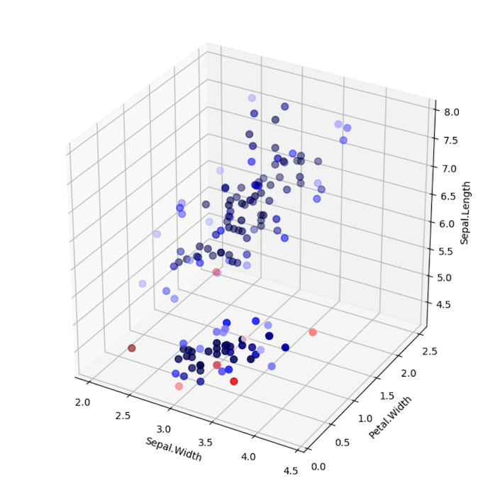
And finally, let's visualize the scores provided by LoOP in both cases (with and without clustering).
fig = plt.figure(figsize=(7, 7))
ax = fig.add_subplot(111, projection='3d')
ax.scatter(iris['Sepal.Width'], iris['Petal.Width'], iris['Sepal.Length'],
c=iris['scores'], cmap='seismic', s=50)
ax.set_xlabel('Sepal.Width')
ax.set_ylabel('Petal.Width')
ax.set_zlabel('Sepal.Length')
plt.show()
plt.clf()
plt.cla()
plt.close()

fig = plt.figure(figsize=(7, 7))
ax = fig.add_subplot(111, projection='3d')
ax.scatter(iris_clust['Sepal.Width'], iris_clust['Petal.Width'], iris_clust['Sepal.Length'],
c=iris_clust['scores'], cmap='seismic', s=50)
ax.set_xlabel('Sepal.Width')
ax.set_ylabel('Petal.Width')
ax.set_zlabel('Sepal.Length')
plt.show()
plt.clf()
plt.cla()
plt.close()

fig = plt.figure(figsize=(7, 7))
ax = fig.add_subplot(111, projection='3d')
ax.scatter(iris_clust['Sepal.Width'], iris_clust['Petal.Width'], iris_clust['Sepal.Length'],
c=iris_clust['labels'], cmap='Set1', s=50)
ax.set_xlabel('Sepal.Width')
ax.set_ylabel('Petal.Width')
ax.set_zlabel('Sepal.Length')
plt.show()
plt.clf()
plt.cla()
plt.close()
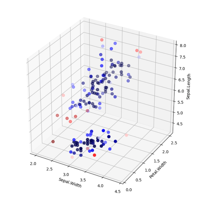
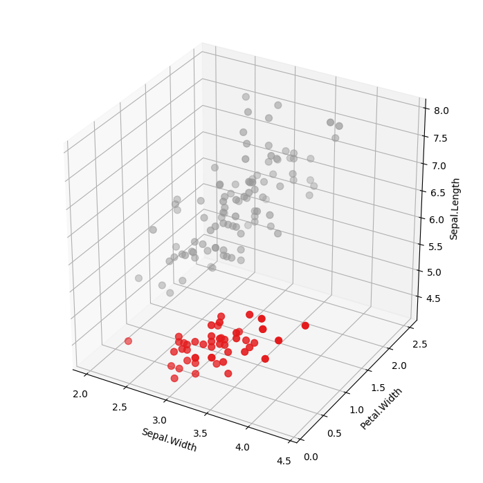
Your results should look like the following:
LoOP Scores without Clustering
LoOP Scores with Clustering
DBSCAN Cluster Assignments
Note the differences between using LocalOutlierProbability with and without clustering. In the example without clustering, samples are
scored according to the distribution of the entire data set. In the example with clustering, each sample is scored
according to the distribution of each cluster. Which approach is suitable depends on the use case.
NOTE: Data was not normalized in this example, but it's probably a good idea to do so in practice.
Using Numpy
When using numpy, make sure to use 2-dimensional arrays in tabular format:
data = np.array([
    [43.3, 30.2, 90.2],
    [62.9, 58.3, 49.3],
    [55.2, 56.2, 134.2],
    [48.6, 80.3, 50.3],
    [67.1, 60.0, 55.9],
    [421.5, 90.3, 50.0]
])

scores = loop.LocalOutlierProbability(data, n_neighbors=3).fit().local_outlier_probabilities
print(scores)
The shape of the input array shape corresponds to the rows (observations) and columns (features) in the data:
print(data.shape)
# (6,3), which matches number of observations and features in the above example
Similar to the above:
data = np.random.rand(100, 5)
scores = loop.LocalOutlierProbability(data).fit().local_outlier_probabilities
print(scores)
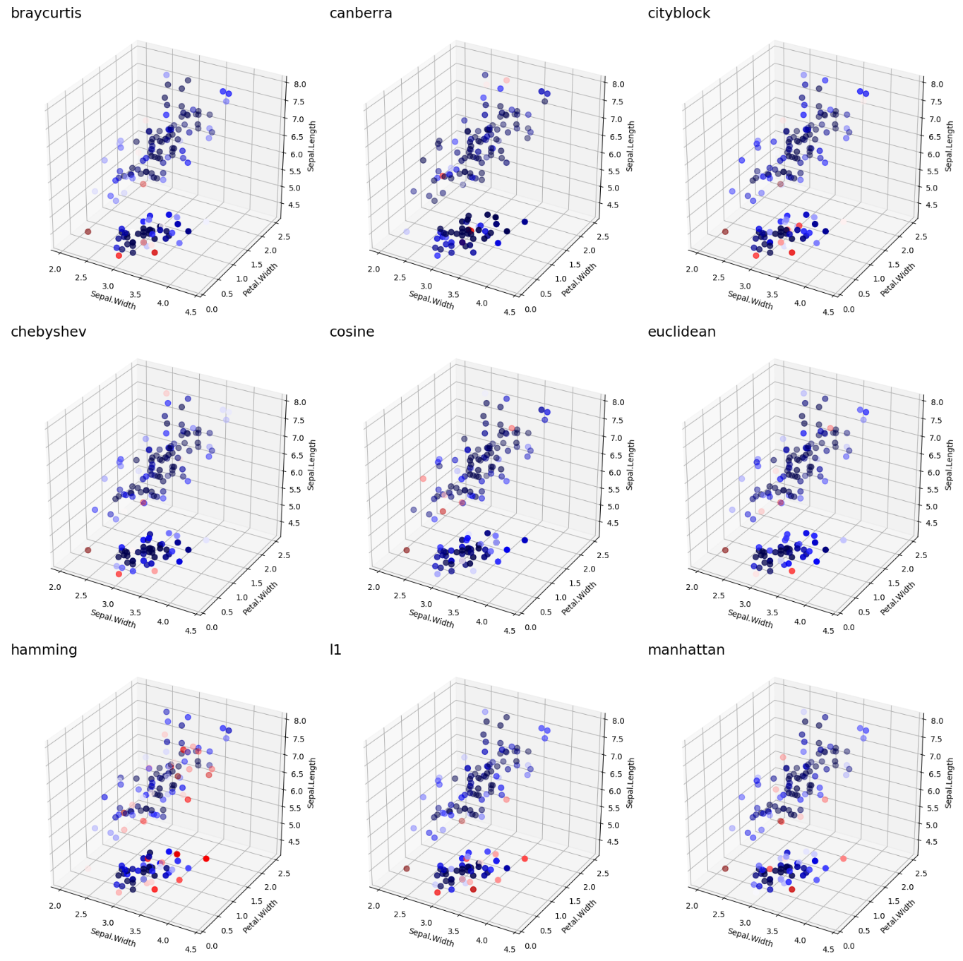
Specifying a Distance Matrix
PyNomaly provides the ability to specify a distance matrix so that any
distance metric can be used (a neighbor index matrix must also be provided).
This can be useful when wanting to use a distance other than the euclidean.
data = np.array([
    [43.3, 30.2, 90.2],
    [62.9, 58.3, 49.3],
    [55.2, 56.2, 134.2],
    [48.6, 80.3, 50.3],
    [67.1, 60.0, 55.9],
    [421.5, 90.3, 50.0]
])

neigh = NearestNeighbors(n_neighbors=3, metric='hamming')
neigh.fit(data)
d, idx = neigh.kneighbors(data, return_distance=True)

m = loop.LocalOutlierProbability(distance_matrix=d, neighbor_matrix=idx, n_neighbors=3).fit()
scores = m.local_outlier_probabilities
The below visualization shows the results by a few known distance metrics:
LoOP Scores by Distance Metric

Streaming Data
PyNomaly also contains an implementation of Hamlet et. al.'s modifications
to the original LoOP approach [4],
which may be used for applications involving streaming data or where rapid calculations may be necessary.
First, the standard LoOP algorithm is used on "training" data, with certain attributes of the fitted data
stored from the original LoOP approach. Then, as new points are considered, these fitted attributes are
called when calculating the score of the incoming streaming data due to the use of averages from the initial
fit, such as the use of a global value for the expected value of the probabilistic distance. Despite the potential
for increased error when compared to the standard approach, but it may be effective in streaming applications where
refitting the standard approach over all points could be computationally expensive.
While the iris dataset is not streaming data, we'll use it in this example by taking the first 120 observations
as training data and take the remaining 30 observations as a stream, scoring each observation
individually.
Split the data.
iris = iris.sample(frac=1) # shuffle data
iris_train = iris.iloc[:, 0:4].head(120)
iris_test = iris.iloc[:, 0:4].tail(30)
Fit to each set.
m = loop.LocalOutlierProbability(iris).fit()
scores_noclust = m.local_outlier_probabilities
iris['scores'] = scores_noclust

m_train = loop.LocalOutlierProbability(iris_train, n_neighbors=10)
m_train.fit()
iris_train_scores = m_train.local_outlier_probabilities
iris_test_scores = []
for index, row in iris_test.iterrows():
    array = np.array([row['Sepal.Length'], row['Sepal.Width'], row['Petal.Length'], row['Petal.Width']])
    iris_test_scores.append(m_train.stream(array))
iris_test_scores = np.array(iris_test_scores)
Concatenate the scores and assess.
iris['stream_scores'] = np.hstack((iris_train_scores, iris_test_scores))
# iris['scores'] from earlier example
rmse = np.sqrt(((iris['scores'] - iris['stream_scores']) ** 2).mean(axis=None))
print(rmse)
The root mean squared error (RMSE) between the two approaches is approximately 0.199 (your scores will vary depending on the data and specification).
The plot below shows the scores from the stream approach.
fig = plt.figure(figsize=(7, 7))
ax = fig.add_subplot(111, projection='3d')
ax.scatter(iris['Sepal.Width'], iris['Petal.Width'], iris['Sepal.Length'],
c=iris['stream_scores'], cmap='seismic', s=50)
ax.set_xlabel('Sepal.Width')
ax.set_ylabel('Petal.Width')
ax.set_zlabel('Sepal.Length')
plt.show()
plt.clf()
plt.cla()
plt.close()
LoOP Scores using Stream Approach with n=10
Notes
When calculating the LoOP score of incoming data, the original fitted scores are not updated.
In some applications, it may be beneficial to refit the data periodically. The stream functionality
also assumes that either data or a distance matrix (or value) will be used across in both fitting
and streaming, with no changes in specification between steps.
Contributing
If you would like to contribute, please fork the repository and make any changes locally prior to submitting a pull request.
Feel free to open an issue if you notice any erroneous behavior.
Versioning
Semantic versioning is used for this project. If contributing, please conform to semantic
versioning guidelines when submitting a pull request.
License
This project is licensed under the Apache 2.0 license.
Research
PyNomaly has been used in the following research:
- Y. Zhao and M.K. Hryniewicki, "XGBOD: Improving Supervised Outlier Detection with Unsupervised Representation Learning," International Joint Conference on Neural Networks (IJCNN), IEEE, 2018.
If your research is missing from this list and should be listed,
please submit a pull request with an addition to the readme.
If citing PyNomaly, use the following:
@article{Constantinou2018,
  doi = {10.21105/joss.00845},
  url = {https://doi.org/10.21105/joss.00845},
  year  = {2018},
  month = {oct},
  publisher = {The Open Journal},
  volume = {3},
  number = {30},
  pages = {845},
  author = {Valentino Constantinou},
  title = {{PyNomaly}: Anomaly detection using Local Outlier Probabilities ({LoOP}).},
  journal = {Journal of Open Source Software}
}


