cLoops2
cLoops2 is an extension of our previous work, cLoops. From loop-calling based on assumption-free clustering to a full suite of analysis tools for 3D genomic interaction data, cLoops2 has been adapted specifically for data such as Hi-TrAC/Trac-looping, for which interactions are enriched over the genome through experimental steps. cLoops2 still supports Hi-C -like data, of which the interaction signals are evenly distributed at enzyme cutting sites. The changes from cLoops to cLoops2 are designed to address challenges around aiming for higher resolutions with the next-generation of genome architecture mapping technologies.
cLoops2 is designed with respect reference to bedtools and Samtools for command-line style programming. If you have experience with them, you will find cLoops2 easy and efficient to use and combine commands, integrate as steps in your processing pipeline.
Please refer to our Hi-TrAC method manuscript or cLoops2 manuscript for what cLoops2 can do and show.
If you use cLoops2 in your research (the idea, the algorithm, the analysis scripts or the supplemental data), please give us a star on the GitHub repo page and cite our paper as follows:
Preprint bioRxiv: Yaqiang Cao et al. "cLoops2: a full-stack comprehensive analytical tool for chromatin interactions"
Install
1. Easy way through pip for stable version
Python3 is requried.
pip install cLoops2
2. Install from source with test data for latest version
cLoops2 is written purely in Python3 (cLoops was written in Python2). If you are familiar with conda, cLoops2 can be installed easily with the following Linux shell commands (also tested well in win10 ubuntu subsystem, MacOS).
# for most updated code, or download the release version
git clone --depth=1 https://github.com/YaqiangCao/cLoops2
cd cLoops2
conda env create --name cLoops2 --file cLoops2_env.yaml
conda activate cLoops2
python3 setup.py install
Necessary Python3 third-party packages are listed below, all of which can be installed through conda. If you like to install cLoops2 through the old school way python setup.py install, please install the 3rd dependencies first.
tqdm
numpy
scipy
pandas
sklearn
seaborn
pyBigWig
matplotlib
joblib
networkx
After installation, whenever you want to run cLoops2, just activate the environment with conda: conda activate cLoops2.
Happy peak/loop-calling and have fun exploring all the other kinds of analyses.
Basic Usage and Quick Guide
Example data background introduction
Example data for testing is available at cLoops2/example/data. The BEDPE files were from Hi-TrAC experiments mapped to hg38 for chromosome 21 in GM12878 and K562 cell lines, two biological replicates for each cell line. Only intra-chromosomal PETs were kept. Raw FASTQ reads were processed by tracPre2.py.
For other kinds of 3D genomic interaction data such as ChIA-PET, Hi-C, and HiChIP, cLoops2 can also start with provided BEDPE files.
The following example command lines were also recorded in cLoops2/example/test_run/run.sh, which can be used to test the main programs of cLoops2 after installation.
Rountine analysis step 1: get basic statistics of PETs from input BEDPE file
cLoops2 qc -f ../data/GM_Trac1_hg38_chr21_partaa.bedpe.gz,../data/GM_Trac1_hg38_chr21_partab.bedpe.gz -o test -p 2
Please note, in cLoops2, multiple files/directories can be assigned as input with the separation of the comma, please do not leave blanks between names. The majority of cLoops2 analysis modules can be run in a parallel way with the option of -p. Most of them will generate a cLoops2.log file recording the program parameters and important messages for later review.
The informative output is a .txt file with annotation of information as follows.
| Sample | TotalPETs | UniquePETs | Redundancy | IntraChromosomalPETs(cis) | cisRatio | InterChromosomalPETs(trans) | transRatio | meanDistance | closePETs(distance<=1kb) | closeRatio | middlePETs(1kb<distance<=10kb) | middleRatio | distalPETs(distance>10kb) | distalRatio |
|---|---|---|---|---|---|---|---|---|---|---|---|---|---|---|
| GM_HiTrac_bio1 | 906506 | 901589 | 0.005424123 | 655640 | 0.727204968 | 245949 | 0.272795032 | 522978.0929 | 138201 | 0.210787932 | 274800 | 0.419132451 | 242639 | 0.370079617 |
| GM_HiTrac_bio2 | 665759 | 662197 | 0.005350284 | 506058 | 0.76421065 | 156139 | 0.23578935 | 501104.2879 | 104360 | 0.206221421 | 216640 | 0.428093223 | 185058 | 0.365685356 |
| K562_HiTrac_bio1 | 596886 | 591215 | 0.009500977 | 474746 | 0.8030006 | 116469 | 0.1969994 | 314420.4126 | 115360 | 0.242993095 | 226568 | 0.477240461 | 132818 | 0.279766444 |
| K562_HiTrac_bio2 | 413818 | 410415 | 0.008223422 | 326743 | 0.796128309 | 83672 | 0.203871691 | 327855.2136 | 68571 | 0.209862185 | 162132 | 0.496206499 | 96040 | 0.293931316 |
Rountine analysis step 2: pre-process BEDPE file(s) into cLoops2 data
#get directory seperately for GM12878, only target chromosome chr21
cLoops2 pre -f ../data/GM_HiTrac_bio1.bedpe.gz -o gm_bio1 -c chr21
cLoops2 pre -f ../data/GM_HiTrac_bio2.bedpe.gz -o gm_bio2 -c chr21
#get the combined data for GM12878
cLoops2 pre -f ../data/GM_HiTrac_bio1.bedpe.gz,../data/GM_HiTrac_bio2.bedpe.gz -o gm -c chr21
#get the directory seperately for K562 first
cLoops2 pre -f ../data/K562_HiTrac_bio1.bedpe.gz -o k562_bio1 -c chr21
cLoops2 pre -f ../data/K562_HiTrac_bio2.bedpe.gz -o k562_bio2 -c chr21
#then combine the data, only keep 1 PET for the same position, default the same to cLoops2 pre
cLoops2 combine -ds k562_bio1,k562_bio2 -o k562 -keep 1
The output directory contains one .json file for the basic PET statistics and .ixy files, which are used to call peaks, loops, or any analysis implemented in cLoops2.
For data backup/sharing purposes, the directory can be saved as a .tar.gz file through tar command.
If you move the directory or change the files in the directory, please run cLoops2 update to update the information of petMeta.json, as all ixy files were recorded as absolute paths.
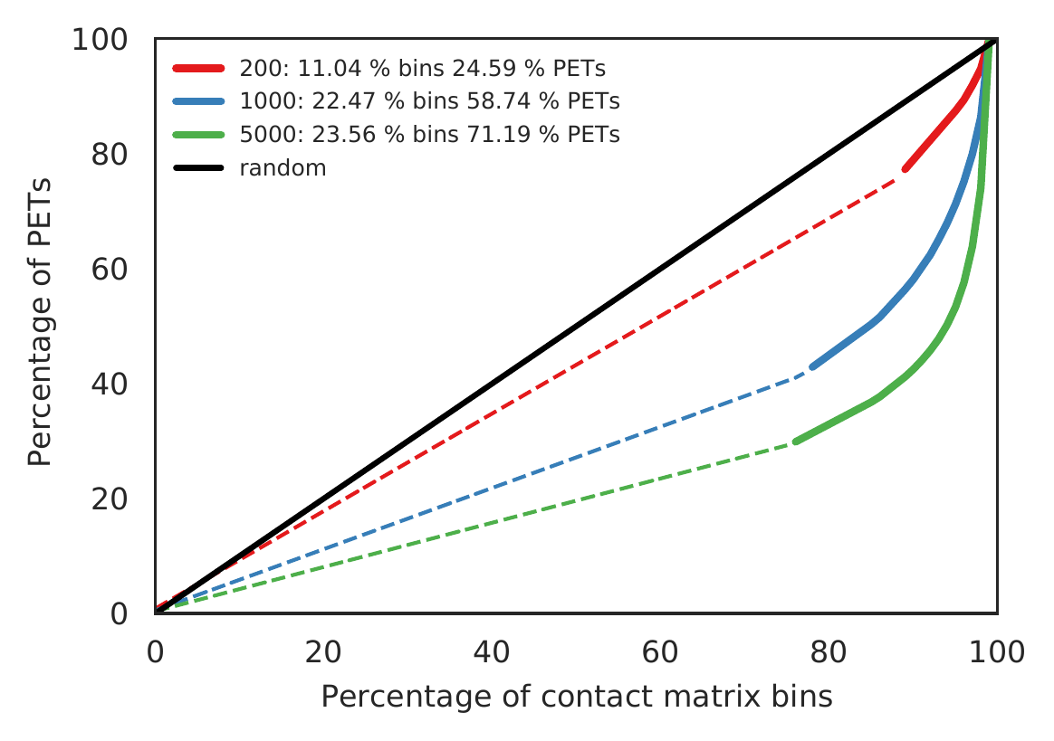
Rountine analysis step 3: estimate reasonable contact matrix resolution
cLoops2 estRes -d gm -o gm -bs 5000,1000,200 -p 10
cLoops2 estRes -d k562 -o k562 -bs 5000,1000,200 -p 10
This step is not needed for peak-calling 1D data such as ChIP-seq or ChIC-seq.
We prefer to use the highest resolution with >=50% PETs (solid lines) for filtering singletons, visualization, or calling loops. Dash lines show the bins with only singleton PETs, evenly distributed so increased stably, higher possibilities of noises.
The main output is a figure as follows.
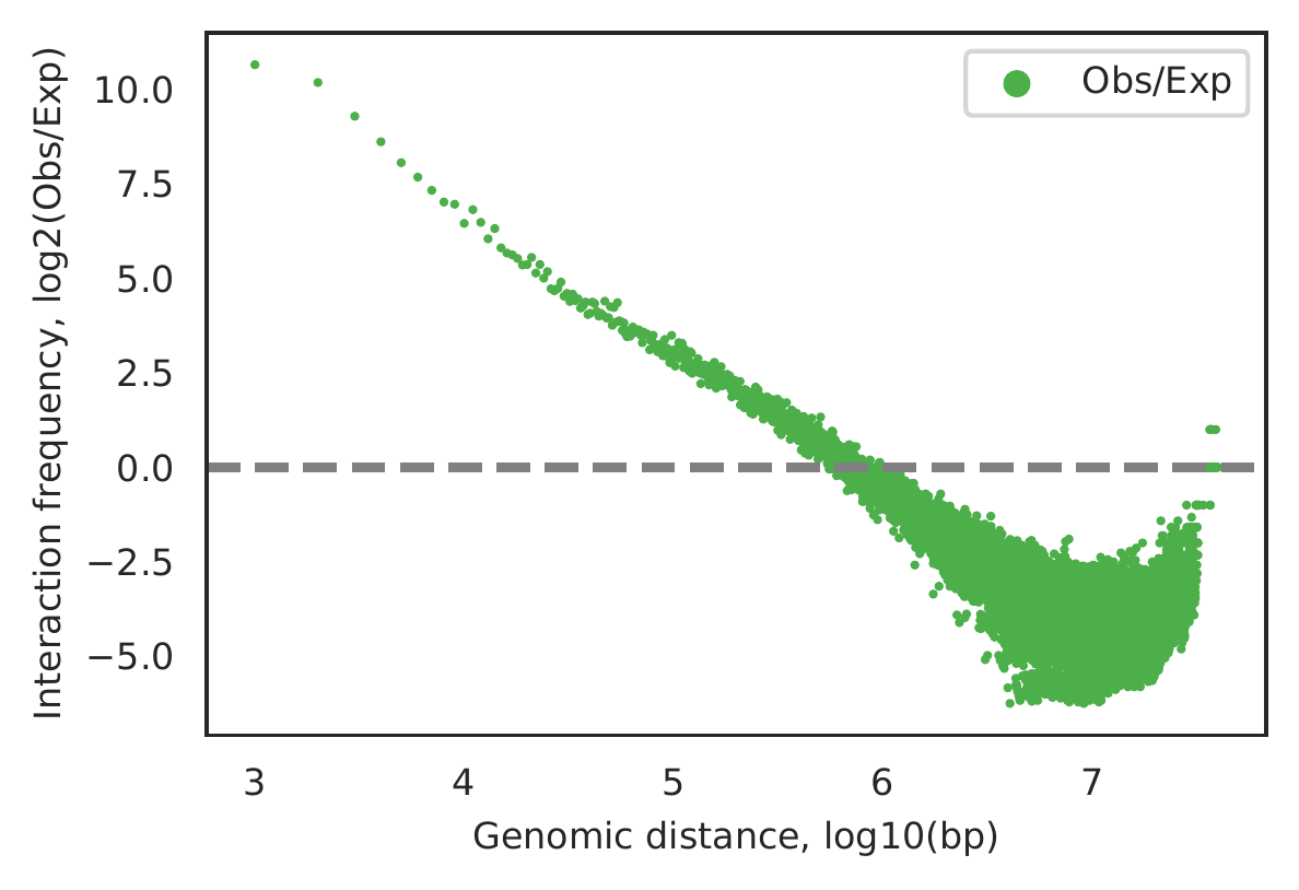
Rountine analysis step 4: estimate significant interaction distance limitation
cLoops2 estDis -d gm -o gm -bs 1000 -p 10 -plot
The main output is a figure as follows. The plot indicates Hi-TrAC data may detect significant interactions within 1MB.
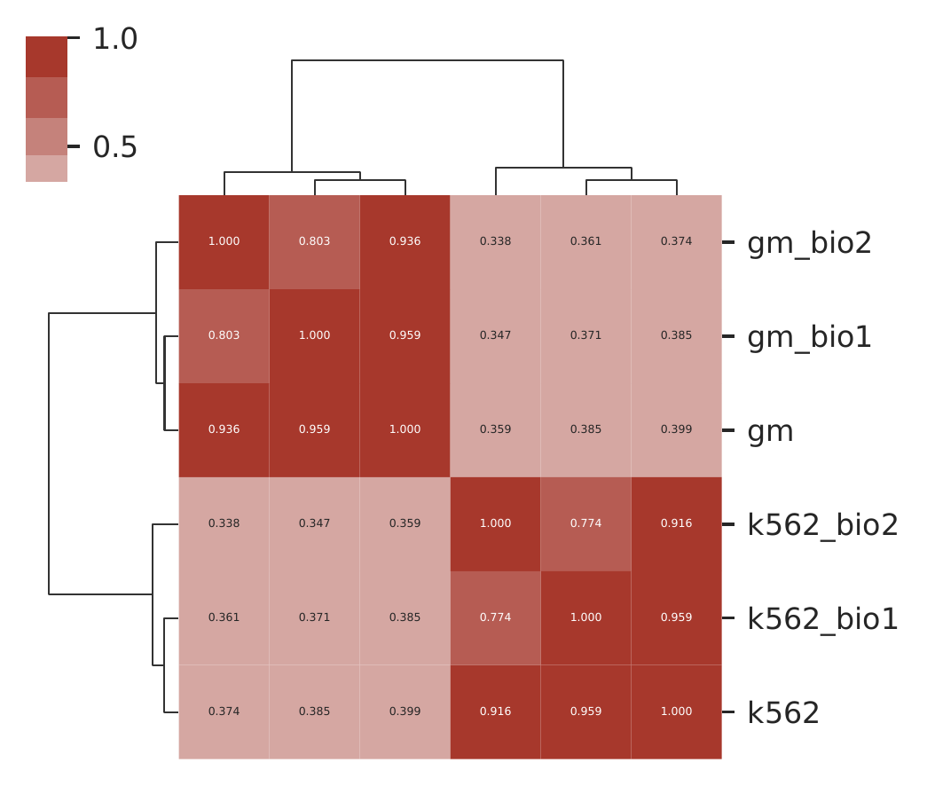
Rountine analysis step 5: estimate similarities/consistency among replicates
cLoops2 estSim -ds gm_bio1,gm_bio2,gm,k562_bio1,k562_bio2,k562 -bs 1000 -plot -p 6 -o test_step4
Rountine analysis step 6: call peaks
Call peaks can be run on raw data or filtered data (through cLoops2 filterPETs), only using PETs within 1kb. Smaller eps, sharper peaks. Run as PETs or split PETs as single-end reads.
cLoops2 callPeaks -d gm -o gm -eps 50,100 -minPts 10 -mcut 1000 -split
The main output is a _peaks.txt file, from which contains all important informations for peaks.
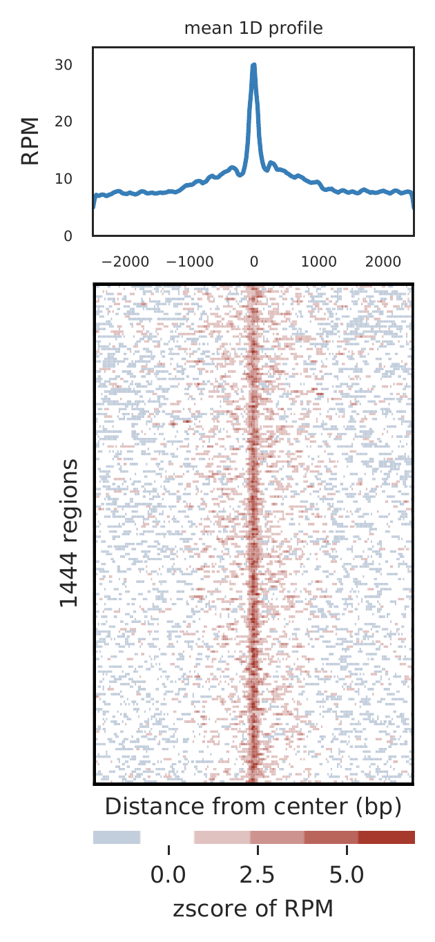
Rountine analysis step 7: show aggregated peaks
Check global peaks width and enrichment through aggregation plot. For Hi-TrAC data, we expect high enrichment of signals at peaks.
cLoops2 agg -d gm -peaks gm_peaks.bed -o gm -peak_ext 2500 -peak_bins 200 -peak_norm -skipZeros
Rountine analysis step 8: call intra-chromosomal loops
Call loops can be run on raw data or filtered data.
#call intra-chromosomal loops, filtered PETs can be used to show clear view of loops, or futhur to call loops
cLoops2 callLoops -d gm -o gm -eps 200,500,1000 -minPts 10 -w -j
The main output is a _loops.txt file, which contains all important information for loops.
We implemented a trans-chromosomal-loops-caller in cLoops callLoops with a parameter of -trans. However, we do not recommend running with this option for Hi-TrAC data.
With the options of -w -j, loops can be output as the input of the washU genome browser and juicebox.
If too many close loops are called, with the option of -max_cut, the maximal distance cutoff for self-ligation PETs vs inter-ligation PETs will be used to filter loops. Also, with the option of -cut, only long-distance PETs will be used to call loops.
With the option of -hic, callLoops will not check the peak-like feature for anchors, more compatible for Hi-C like data.
Because in cLoops2 the backend clustering algorithm is different from that of cLoops, so even the same parameter may have different results.
Rountine analysis step 9: show aggregated loops
cLoops2 agg -d gm -o gm -loops gm_loops.txt -bws ../data/GM12878_ATAC_chr21.bw,../data/GM12878_CTCF_chr21.bw -1D -loop_norm
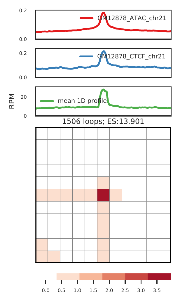
For Hi-TrAC, we expect the aggregated loops pattern as above:
- highly enriched signal at the center for loop regions;
- relative higher signal from the two anchors, as for Hi-TrAC, anchors are expected to be peaks in the 1D.
Rountine analysis step 10: call domains
cLoops2 callDomains -d gm -o gm -bs 5000 -ws 100000,250000
The main output is a _domains.txt file.
For Hi-TrAC, called domains are all activate domains. There is a -hic option for Hi-C like data.
Rountine analysis step 11: show aggregated domains
#convert the output segregation score from bedGraph file to bigWig
bedGraphToBigWig  gm_domains_SS_binSize5.0k_winSize100.0k.bdg ../../data/hg38.chrom.sizes gm_domains_SS_bs5k_ws100k.bw
bedGraphToBigWig  gm_domains_SS_binSize5.0k_winSize250.0k.bdg ../../data/hg38.chrom.sizes gm_domains_SS_bs5k_ws250k.bw
cLoops2 agg -d gm -o gm -domains gm_domains.bed -bws ../data/GM12878_CTCF_chr21.bw,gm_domains_SS_bs5k_ws100k.bw,gm_domains_SS_bs5k_ws250k.bw -1D
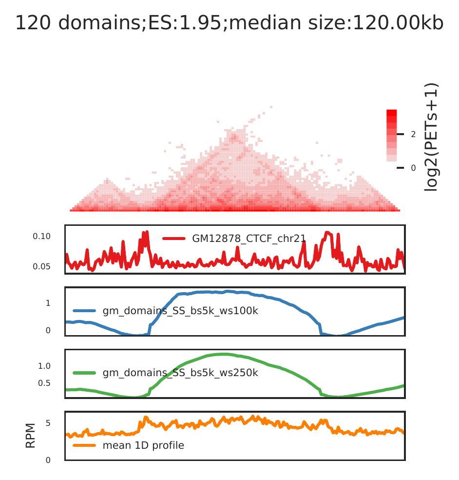
For Hi-TrAC, we expect the aggregated domains pattern as above (maybe better clear if there are more domains):
- clear segregation from up-and down-stream;
- enriched CTCF/Cohesin bindings at boundaries;
- higher 1D signal than nearby regions;
- small domains.
Rountine analysis step 12: visualization
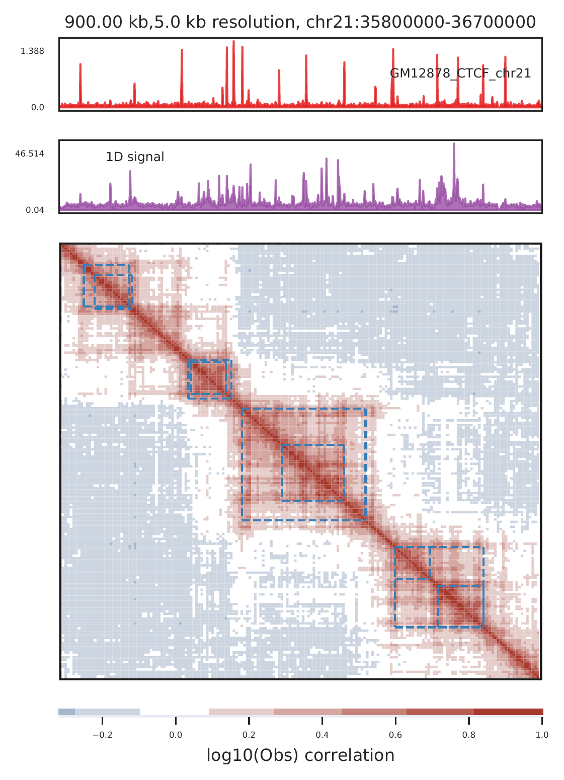
cLoops2 plot can show the interaction contact matrix (observed, observed/expected, correlation) at any resolution, with genes (-gtf option), 1D annotations (-bws option), domains (-dominas option), loops (-loops option).
a.show big regions such as domains
cLoops2 plot -f ./gm/chr21-chr21.ixy -o gm_domain_example -bs 5000 -start 35830000 -end 36950000 -domains gm_domains.bed -log -bws ../data/GM12878_CTCF_chr21.bw -1D -corr
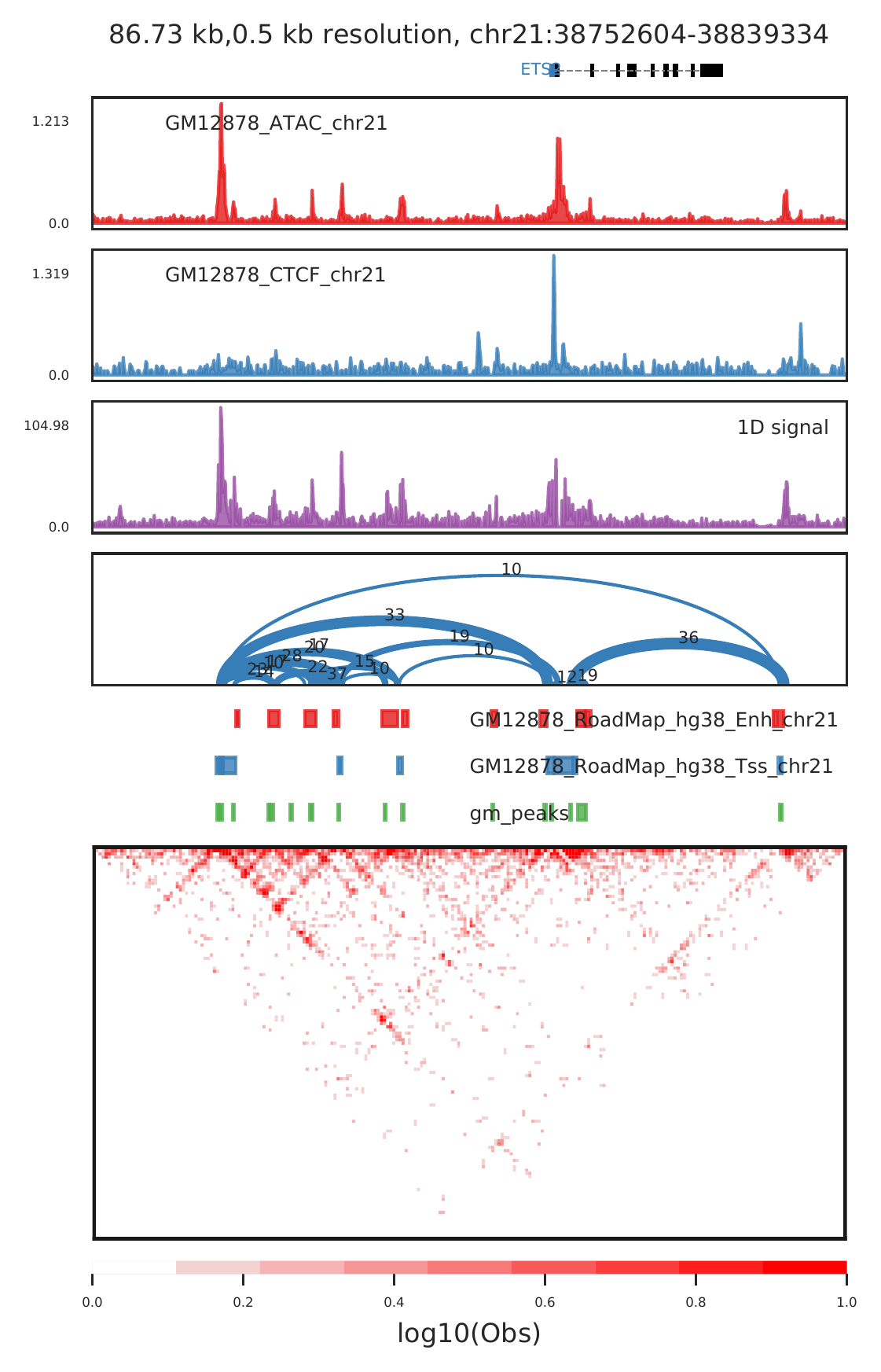
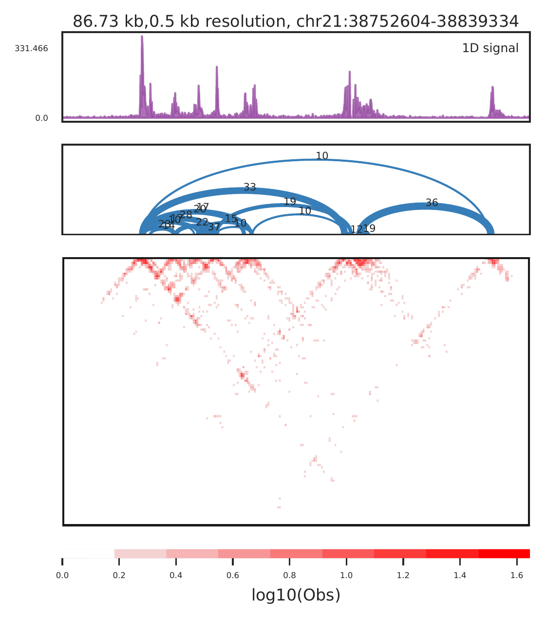
b.show small regions such as peaks and loops
#show enhancer-promoter loops
cLoops2 plot -f gm/chr21-chr21.ixy -o gm_example -bs 500 -start 38752604 -end 38839334 -triu -bw ../data/GM12878_ATAC_chr21.bw,../data/GM12878_CTCF_chr21.bw -1D -loops gm_loops.txt -beds ../data/GM12878_RoadMap_hg38_Enh_chr21.bed,../data/GM12878_RoadMap_hg38_Tss_chr21.bed,gm_peaks.bed -m obs -log -gtf ../data/gencode_v30_chr21.gtf -vmax 1
The raw data can be further filtered by loops (or peaks) to show much better view.
cLoops2 filterPETs -d gm -loops gm_loops.txt -o gm_filtered
cLoops2 plot -f gm_filtered/chr21-chr21.ixy -o gm_filtered_example -bs 500 -start 38752604 -end 38839334 -triu -loops gm_loops.txt -log -1D
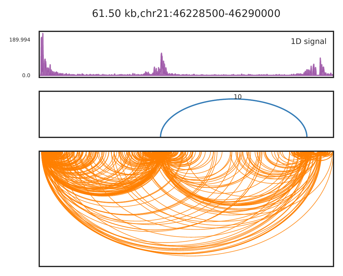
For close loops, we also recommend to use -arch mode, to show raw PETs as arches for called loops. Better for checking the anchor locations and interaction densities compared to nearby backgroud.
cLoops2 plot -f gm_filtered/chr21-chr21.ixy -o gm_example -start 46228500 -end 46290000 -1D -loops gm_loops.txt -arch -aw 0.05
Rountine analysis step 13: call differential enriched loops for two conditions
#a. sampling PETs to same/similar depth to call loops with same parameters
cLoops2 samplePETs -d gm -o gm_samp -tot 780000
cLoops2 samplePETs -d k562 -o k562_samp -tot 780000
#b. call loops with same parameters
cLoops2 callLoops -d gm_samp -o gm_samp -eps 200,500,1000 -minPts 10 -w -j
cLoops2 callLoops -d k562_samp -o k562_samp -eps 200,500,1000 -minPts 10 -w -j
#c. call differentially enriched loops
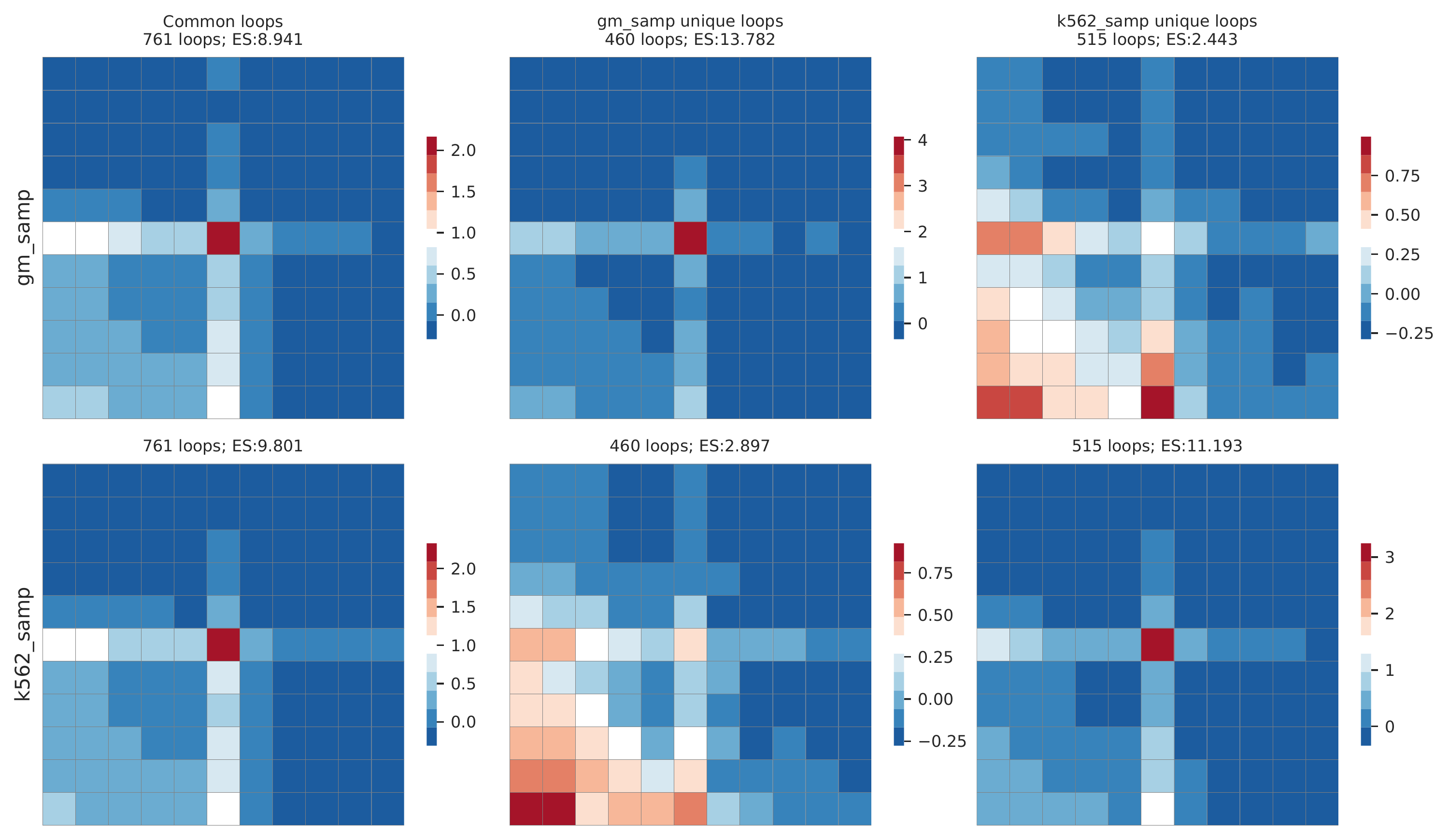
cLoops2 callDiffLoops -tloop gm_samp_loops.txt -td gm_samp -cloop k562_samp_loops.txt -cd k562_samp -o gm_vs_k562 -j -w
The main output is a _dloops.txt file with three figures. The most import figure shows the aggregated features of called common and specific loops.
Rountine analysis step 14: convert cLoops2 data to others
More formats will be added if actually needed.
1. to BED file
cLoops2 dump -d gm -o gm -bed
2. to BEDPE file
cLoops2 dump -d gm -o gm -bedpe
3. interaction data to bedGraph file
cLoops2 dump -d gm -o gm -bdg
4. ChIP-seq -like data to bedGraph file
cLoops2 dump -d gm -o gm -bdg_pe
5. to washU genome browser long-range interaction track
cLoops2 dump -d gm -o gm -washU
6. to HIC file, juicer_tools need in command line envrionment
cLoops2 dump -d gm -o gm -hic -hic_org hg38 -hic_res 200000,25000,5000
7. to TXT file of contact matrix
cLoops2 dump -d gm -mat -o gm -mat_res 10000 -mat_chrom chr21-chr21 -mat_start 36000000 -mat_end 40000000 -log -norm -corr
Rountine analysis step 15: quantify features from cLoops2 data
1. quantify GM12878 peaks in K562 data
cLoops2 quant -d k562 -peaks gm_peaks.bed -o k562_gm
2. quantify GM12878 loops in K562 data
cLoops2 quant -d k562 -loops gm_loops.txt -o k562_gm
3. quantify GM12878 domains in K562 data
#key parameteres of -bs and -ws from cLoops2 callDomains needed
cLoops2 quant -d k562 -domains gm_domains.txt -o k562_gm -domain_bs 5000 -domain_ws 100000
Rountine analysis step 16: montage analysis of interactions among distal genomic regions
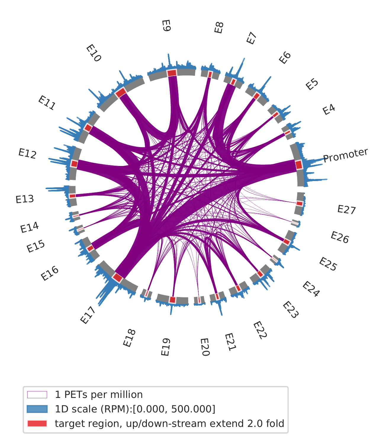
1. show all interactions among enhancers and promoters
cLoops2 montage -f ./gm_samp/chr21-chr21.ixy -bed ../data/runx1.bed -o gm_runx1_all -ext 2 -simple -ppmw 0.05 -vmax 500
cLoops2 montage -f ./k562_samp/chr21-chr21.ixy -bed ../data/runx1.bed -o k562_runx1_all -ext 2 -simple -ppmw 0.05 -vmax 500
| GM12878 | K562 |
|---|---|
 |
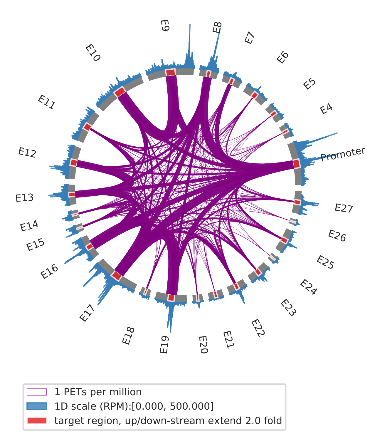 |
2. show interactions for slected view points, such as one enhancer and promoter
cLoops2 montage -f ./gm_samp/chr21-chr21.ixy -bed ../data/runx1.bed -o gm_runx1_vp -ext 2 -simple -ppmw 0.05 -vmax 500 -vp Promoter,E19
cLoops2 montage -f ./k562_samp/chr21-chr21.ixy -bed ../data/runx1.bed -o k562_runx1_vp -ext 2 -simple -ppmw 0.05 -vmax 500 -vp Promoter,E19
| GM12878 | K562 |
|---|---|
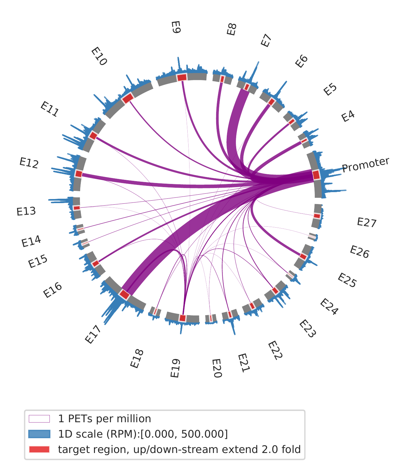 |
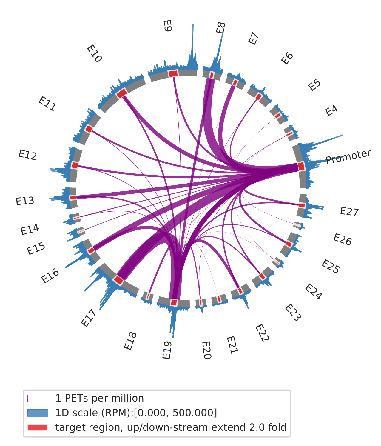 |
Rountine analysis step 17: annotate loops to genes and find a gene's all interacting enhancers
cLoops2 anaLoops -loop gm_loops.txt -o gm_loops -gtf ../data/gencode_v30_chr21.gtf -net
There will be 5 files for the -gtf -net option as following.
- _LoopsGtfAno.txt file for main annotations. Loop anchors were assigned to gene promoters and enhancers based on distance. If only run with -gtf option, this file is the only result.
- _mergedAnchors.txt file for merged anchors. There will also be a _nergedAnchors.bed file converted as bed file for convenience loading to genome browser.
- _loop2anchors.txt file for loops to merged anchors.
- _targets.txt file for every promoter's interacting enhancer and promoter. If there are >=2 enhancers/promoters linked, HITS algorithm will be used to find the hubs. Montage analysis can be followed to show interactions for a specific promoter.
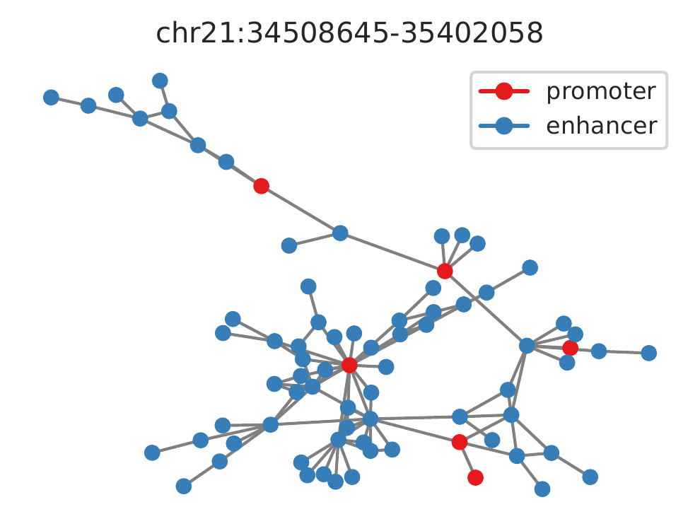
- _ep_net.sif: SIF file for interactions networks of annotated enhancers and promoters, can be loaded in Cytoscape for visualization. Can be further used to analyze the topological structures of enhancers and promoters.
For example, visualization of the largest connected components for annotated enhancers and promoters.
#just use to show network example, not very pretty one.
#Can be further imporoved, for example, node size can show the accessibility level.
python plotNetExample.py
cLoops2 Main Functions
Run cLoops2 or cLoops2 -h can show the main functions of cLoops2 with short descriptions and examples.
An enhanced, accurate and flexible peak/domain/loop-calling and analysis tool
for 3D genomic interaction data.

Use cLoops2 sub-command -h to see detail options and examples for sub-commands.
Available sub-commands are:
    qc: quality control of BEDPE files before analysis.
    pre: preprocess input BEDPE files into cLoops2 data.
    update: update cLoops2 data files locations.
    combine: combine multiple cLooops2 data directories.
    dump: convert cLoops2 data files to others (BEDPE, HIC, washU, bedGraph and
          contact matrix)
    estEps: estimate eps using Gaussian mixture models or k-distance plot.
    estRes: estimate reasonable contact matrix resolution based on signal
            enrichment.
    estDis: estimate significant interactions distance range.
    estSat: estimate sequencing saturation based on contact matrix.
    estSim: estimate similarities among samples based on contact matrix.
    filterPETs: filter PETs based on peaks, loops, singleton mode or knn mode.
    samplePETs: sample PETs according to specific target size.
    callPeaks: call peaks for ChIP-seq, ATAC-seq, ChIC-seq and CUT&Tag or the
               3D genomic data such as Trac-looping, Hi-TrAC, HiChIP and more.
    callLoops: call loops for 3D genomic data.
    callDiffLoops: call differentially enriched loops for two datasets.
    callDomains: call domains for 3D genomic data.
    plot: plot the interaction matrix, genes, view point plot, 1D tracks,
          peaks, loops and domains for a specific region.
    montage: analysis of specific regions, producing Westworld Season 3 -like
             Rehoboam plot.
    agg: aggregated feature analysis and plots, features can be peaks, view
         points, loops and domains.
    quant: quantify peaks, loops and domains.
    anaLoops: anotate loops for target genes.
    findTargets: find target genes of genomic regions through networks from
                 anaLoops.

Examples:
    cLoops2 qc -f trac_rep1.bedpe.gz,trac_rep2.bedpe,trac_rep3.bedpe.gz \
               -o trac_stat -p 3
    cLoops2 pre -f ../test_GM12878_chr21_trac.bedpe -o trac
    cLoops2 update -d ./trac
    cLoops2 combine -ds ./trac1,./trac2,./trac3 -o trac_combined -keep 1
    cLoops2 dump -d ./trac -o trac -hic
    cLoops2 estEps -d trac -o trac_estEps_gmm -p 10 -method gmm
    cLoops2 estRes -d trac -o trac_estRes -p 10 -bs 25000,5000,1000,200
    cLoops2 estDis -d trac -o trac -plot -bs 1000
    cLoops2 estSim -ds Trac1,Trac2 -o trac_sim -p 10 -bs 2000 -m pcc -plot
    cLoops2 filterPETs -d trac -peaks trac_peaks.bed -o trac_peaksFiltered -p 10
    cLoops2 samplePETs -d trac -o trac_sampled -t 5000000 -p 10
    cLoops2 callPeaks -d H3K4me3_ChIC -bgd IgG_ChIC -o H3K4me3_cLoops2 -eps 150 \
                      -minPts 10
    cLoops2 callLoops -d Trac -eps 200,500,1000 -minPts 3 -filter -o Trac -w -j \
                      -cut 2000
    cLoops2 callLoops -d HiC -eps 1000,5000,10000 -minPts 10,20,50,100 -w -j \
                      -trans -o HiC_trans
    cLoops2 callDiffLoops -tloop target_loop.txt -cloop control_loop.txt \
                          -td ./target -cd ./control -o target_diff
    cLoops2 callDomains -d trac -o trac -bs 10000 -ws 200000
    cLoops2 plot -f test/chr21-chr21.ixy -o test -bs 500 -start 34840000 \
                 -end 34895000 -triu -1D -loop test_loops.txt -log \
                 -gtf hg38.gtf -bws ctcf.bw -beds enhancer.bed
    cLoops2 montage -f test/chr21-chr21.ixy -o test -bed test.bed
    cLoops2 agg -d trac -loops trac.loop -peaks trac_peaks.bed \
                -domains hic_domains.bed -bws CTCF.bw,ATAC.bw -p 20 -o trac
    cLoops2 quant -d trac -peaks trac_peaks.bed -loops trac.loop \
                  -domains trac_domain.txt -p 20 -o trac
    cLoops2 anaLoops -loops test_loop.txt -gtf gene.gtf -net -o test
    cLoops2 findTargets -net test_ep_net.sif -tg test_targets.txt \
                        -bed GWAS.bed -o test
    More usages and examples are shown when run with cLoops2 sub-command -h.


optional arguments:
  -h, --help  show this help message and exit
  -d PREDIR   Assign data directory generated by cLoops2 pre to carry out analysis.
  -o FNOUT    Output data directory / file name prefix, default is cLoops2_output.
  -p CPU      CPUs used to run the job, default is 1, set -1 to use all CPUs
              available. Too many CPU could cause out-of-memory problem if there are
              too many PETs.
  -cut CUT    Distance cutoff to filter cis PETs, only keep PETs with distance
              >=cut. Default is 0, no filtering.
  -mcut MCUT  Keep the PETs with distance <=mcut. Default is -1, no filtering.
  -v          Show cLoops2 verison number and exit.
  ---         Following are sub-commands specific options. This option just show
              version of cLoops2.

Bug reports are welcome and can be put as issue at github repo or sent to
[email protected] or [email protected]. Thank you.
1. Quality control for BEDPE files
Run cLoops2 qc -h to see details.
Get the basic quality control statistical information from interaction BEDPE
files.

Example:
    cLoops2 qc -f trac_rep1.bedpe.gz,trac_rep2.bedpe,trac_rep3.bedpe.gz -p 3 \
               -o trac_stat


optional arguments:
  -h, --help  show this help message and exit
  -d PREDIR   Assign data directory generated by cLoops2 pre to carry out analysis.
  -o FNOUT    Output data directory / file name prefix, default is cLoops2_output.
  -p CPU      CPUs used to run the job, default is 1, set -1 to use all CPUs
              available. Too many CPU could cause out-of-memory problem if there are
              too many PETs.
  -cut CUT    Distance cutoff to filter cis PETs, only keep PETs with distance
              >=cut. Default is 0, no filtering.
  -mcut MCUT  Keep the PETs with distance <=mcut. Default is -1, no filtering.
  -v          Show cLoops2 verison number and exit.
  ---         Following are sub-commands specific options. This option just show
              version of cLoops2.
  -f FNIN     Input BEDPE file(s), .bedpe and .bedpe.gz are both suitable. Multiple
              samples can be assigned as -f A.bedpe.gz,B.bedpe.gz,C.bedpe.gz.
2. Pre-process BEDPE into cLoops2 data
Run cLoops2 pre -h to see details.
Preprocess BEDPE PETs into cLoops2 data files.

The output directory contains one .json file for the basic statistics of PETs
information and .ixy files which are coordinates for every PET. The coordinate
files will be used to call peaks, loops or any other analyses implemented in
cLoops2. For data backup/sharing purposes, the directory can be saved as
.tar.gz file through tar. If changed and moved location, run
***cLoops2 update -d*** to update.

Examples:
    1. keep high quality PETs of chromosome chr21
        cLoops2 pre -f trac_rep1.bepee.gz,trac_rep2.bedpe.gz -o trac -c chr21

    2. keep all cis PETs that have distance > 1kb
        cLoops2 pre -f trac_rep1.bedpe.gz,trac_rep2.bedpe.gz -o trac -mapq 0


optional arguments:
  -h, --help  show this help message and exit
  -d PREDIR   Assign data directory generated by cLoops2 pre to carry out analysis.
  -o FNOUT    Output data directory / file name prefix, default is cLoops2_output.
  -p CPU      CPUs used to run the job, default is 1, set -1 to use all CPUs
              available. Too many CPU could cause out-of-memory problem if there are
              too many PETs.
  -cut CUT    Distance cutoff to filter cis PETs, only keep PETs with distance
              >=cut. Default is 0, no filtering.
  -mcut MCUT  Keep the PETs with distance <=mcut. Default is -1, no filtering.
  -v          Show cLoops2 verison number and exit.
  ---         Following are sub-commands specific options. This option just show
              version of cLoops2.
  -f FNIN     Input BEDPE file(s), .bedpe and .bedpe.gz are both suitable.
              Replicates or multiple samples can be assigned as -f A.bedpe.gz,
              B.bedpe.gz,C.bedpe.gz to get merged PETs.
  -c CHROMS   Argument to process limited set of chromosomes, specify it as chr1,
              chr2,chr3. Use this option to filter reads from such as
              chr22_KI270876v1. The default setting is to use the entire set of
              chromosomes from the data.
  -trans      Whether to parse trans- (inter-chromosomal) PETs. The default is to
              ignore trans-PETs. Set this flag to pre-process all PETs.
  -mapq MAPQ  MAPQ cutoff to filter raw PETs, default is >=10.
3. Update cLoops2 data directory
Run cLoops2 update -h to see details.
Update cLoops2 data files generated by **cLoops2 pre**.

In the **cLoops2 pre** output directory, there is a .json file annotated with
the .ixy **absolute paths** and other information. So if the directory is
moved, or some .ixy files are removed or changed, this command is needed to
update the paths, otherwise the other analysis modules will not work.

Example:
    cLoops2 update -d ./Trac


optional arguments:
  -h, --help  show this help message and exit
  -d PREDIR   Assign data directory generated by cLoops2 pre to carry out analysis.
  -o FNOUT    Output data directory / file name prefix, default is cLoops2_output.
  -p CPU      CPUs used to run the job, default is 1, set -1 to use all CPUs
              available. Too many CPU could cause out-of-memory problem if there are
              too many PETs.
  -cut CUT    Distance cutoff to filter cis PETs, only keep PETs with distance
              >=cut. Default is 0, no filtering.
  -mcut MCUT  Keep the PETs with distance <=mcut. Default is -1, no filtering.
  -v          Show cLoops2 verison number and exit.
  ---         Following are sub-commands specific options. This option just show
              version of cLoops2.
4. Convert cLoops2 data to others
Run cLoops2 dump -h to see details.
Convert cLoops2 data files to other types. Currently supports BED file,BEDPE
file, HIC file, washU long-range track, bedGraph file and matrix txt file.

Converting cLoops2 data to .hic file needs "juicer_tools pre" in the command
line enviroment.
Converting cLoops2 data to legacy washU browser long-range track needs bgzip
and tabix. Format reference: http://wiki.wubrowse.org/Long-range.
Converting cLoops2 data to UCSC bigInteract track needs bedToBigBed. Format
reference: https://genome.ucsc.edu/goldenPath/help/interact.html.
Converting cLoops2 data to bedGraph track will normalize value as RPM
(reads per million). Run with -bdg_pe flag for 1D data such as ChIC-seq,
ChIP-seq and ATAC-seq.
Converting cLoops2 data to matrix txt file will need specific resolution.
The output txt file can be loaded in TreeView for visualization or further
analysis.

Examples:
    1. convert cLoops2 data to single-end .bed file fo usage of BEDtools or
       MACS2 for peak-calling with close PETs
        cLoops2 dump -d trac -o trac -bed -mcut 1000

    2. convert cLoops2 data to .bedpe file for usage of BEDtools, only keep
       PETs distance >1kb and < 1Mb
        cLoops2 dump -d trac -o trac -bedpe -bedpe_ext -cut 1000 -mcut 1000000

    3. convert cLoops2 data to .hic file to load in juicebox
        cLoops2 dump -d trac -o trac -hic -hic_org hg38 \
                    -hic_res 200000,20000,5000

    4. convert cLoops2 data to washU long-range track file, only keep PETs
       distance > 1kb
        cLoops2 dump -d trac -o trac -washU -washU_ext 50 -cut 1000

    5. convert cLoops2 data to UCSC bigInteract track file
        cLoops2 dump -d trac -o trac -ucsc -ucsc_cs ./hg38.chrom.sizes

    6. convert interacting cLoops2 data to bedGraph file with all PETs
        cLoops2 dump -d trac -o trac -bdg -bdg_ext 100

    7. convert 1D cLoops2 data (such as ChIC-seq/ChIP-seq/ATAC-seq) to bedGraph
       file
        cLoops2 dump -d trac -o trac -bdg -pe

    8. convert 3D cLoops2 data (such as Trac-looping) to bedGraph file for peaks
        cLoops2 dump -d trac -o trac -bdg -mcut 1000

    9. convert one region in chr21 to contact matrix correlation matrix txt file
        cLoops2 dump -d test -mat -o test -mat_res 10000 \
                    -mat_chrom chr21-chr21 -mat_start 36000000 \
                    -mat_end 40000000 -log -corr


optional arguments:
  -h, --help            show this help message and exit
  -d PREDIR             Assign data directory generated by cLoops2 pre to carry out analysis.
  -o FNOUT              Output data directory / file name prefix, default is cLoops2_output.
  -p CPU                CPUs used to run the job, default is 1, set -1 to use all CPUs
                        available. Too many CPU could cause out-of-memory problem if there are
                        too many PETs.
  -cut CUT              Distance cutoff to filter cis PETs, only keep PETs with distance
                        >=cut. Default is 0, no filtering.
  -mcut MCUT            Keep the PETs with distance <=mcut. Default is -1, no filtering.
  -v                    Show cLoops2 verison number and exit.
  ---                   Following are sub-commands specific options. This option just show
                        version of cLoops2.
  -bed                  Convert data to single-end BED file.
  -bed_ext BED_EXT      Extension from the center of the read to both ends for BED file.
                        Default is 50.
  -bedpe                Convert data to BEDPE file.
  -bedpe_ext BEDPE_EXT  Extension from the center of the PET to both ends for BEDPE file.
                        Default is 50.
  -hic                  Convert data to .hic file.
  -hic_org HIC_ORG      Organism required to generate .hic file,default is hg38. If the
                        organism is not available, assign a chrom.size file.
  -hic_res HIC_RES      Resolutions used to generate .hic file. Default is 1000,5000,25000,
                        50000,100000,200000.
  -washU                Convert data to legacy washU browser long-range track.
  -washU_ext WASHU_EXT  Extension from the center of the PET to both ends for washU track.
                        Default is 50.
  -ucsc                 Convert data to UCSC bigInteract file track.
  -ucsc_ext UCSC_EXT    Extension from the center of the PET to both ends for ucsc
                        track. Default is 50.
  -ucsc_cs UCSC_CS      A chrom.sizes file. Can be obtained through fetchChromSizese.
                        Required for -ucsc option.
  -bdg                  Convert data to 1D bedGraph track file.
  -bdg_ext BDG_EXT      Extension from the center of the PET to both ends for
                        bedGraph track. Default is 50.
  -bdg_pe               When converting to bedGraph, argument determines whether to treat PETs
                        as ChIP-seq, ChIC-seq or ATAC-seq paired-end libraries. Default is not.
                        PETs are treated as single-end library for interacting data.
  -mat                  Convert data to matrix txt file with required resolution.
  -mat_res MAT_RES      Bin size/matrix resolution (bp) to generate the contact matrix.
                        Default is 5000 bp.
  -mat_chrom CHROM      The chrom-chrom set will be processed. Specify it as chr1-chr1.
  -mat_start START      Start genomic coordinate for the target region. Default will be the
                        smallest coordinate from specified chrom-chrom set.
  -mat_end END          End genomic coordinate for the target region. Default will be the
                        largest coordinate from specified chrom-chrom set.
  -log                  Whether to log transform the matrix. Default is not.
  -m {obs,obs/exp}      The type of matrix, observed matrix or observed/expected matrix,
                        expected matrix will be generated by shuffling PETs. Default is
                        observed.
  -corr                 Whether to get the correlation matrix. Default is not.
  -norm                 Whether to normalize the matrix with z-score. Default is not.
5. Estimate eps
Run cLoops2 estEps -h to see details.
Estimate key parameter eps.

Two methods are implemented: 1) unsupervised Gaussian mixture model (gmm), and
2) k-distance plot (k-dis,-k needed). Gmm is based on the assumption that PETs
can be classified into self-ligation (peaks) and inter-ligation (loops). K-dis
is based on the k-nearest neighbors distance distribution to find the "knee",
which is where the distance (eps) between neighbors has a sharp increase along
the k-distance curve. K-dis is the traditional approach literatures, but it is
much more time consuming than gmm, and maybe only fit to small cases. If both
methods do not give nice plots, please turn to the empirical parameters you
like, such as 100,200 for ChIP-seq -like data, 5000,1000 for Hi-C and etc.

Examples:
    1. estimate eps with Gaussian mixture model
        cLoops2 estEps -d trac -o trac_estEps_gmm -p 10 -method gmm

    2. estimate eps with k-nearest neighbors distance distribution
        cLoops2 estEps -d trac -o trac_estEps_kdis -p 10 -method k-dis -k 5


optional arguments:
  -h, --help           show this help message and exit
  -d PREDIR            Assign data directory generated by cLoops2 pre to carry out analysis.
  -o FNOUT             Output data directory / file name prefix, default is cLoops2_output.
  -p CPU               CPUs used to run the job, default is 1, set -1 to use all CPUs
                       available. Too many CPU could cause out-of-memory problem if there are
                       too many PETs.
  -cut CUT             Distance cutoff to filter cis PETs, only keep PETs with distance
                       >=cut. Default is 0, no filtering.
  -mcut MCUT           Keep the PETs with distance <=mcut. Default is -1, no filtering.
  -v                   Show cLoops2 verison number and exit.
  ---                  Following are sub-commands specific options. This option just show
                       version of cLoops2.
  -fixy FIXY           Assign the .ixy file to estimate eps inside of the whole directory
                       generated by cLoops2 pre. For very large data, especially Hi-C, this
                       option is recommended for chr1 (or the smaller one) to save time.
  -k KNN               The k-nearest neighbors used to draw the k-distance plot. Default is 0
                       (not running), set this when -method k-dis. Suggested 5 for
                       ChIA-PET/Trac-looping data, 20 or 30 for Hi-C like data.
  -method {gmm,k-dis}  Two methods can be chosen to estimate eps. Default is Gmm. See above
                       for difference of the methods.
6. Estimate reasonable contact matrix resolution
Run cLoops2 estRes -h to see details.
Estimate reasonable genome-wide contact matrix resolution based on signal
enrichment.

PETs will be assigned to contact matrix bins according to input resolution. A
bin is marked as [nx,ny], and a PET is assigned to a bin by nx = int((x-s)/bs),
ny = int((y-s)/bs), where s is the minimal coordinate for all PETs and bs is
the bin size. Self-interaction bins (nx=ny) will be ignored. The bins only
containing singleton PETs are assumed as noise.

The output is a PDF plot, for each resolution, a line is separated into two
parts: 1) dash line indicated linear increased trend of singleton PETs/bins; 2)
solid thicker line indicated non-linear increased trend of higher potential
signal PETs/bins. The higher the ratio of signal PETs/bins, the easier it it to
find loops in that resolution. The closer to the random line, the higher the
possibility to observe evenly distributed signals.

We expect the highest resolution with >=50% PETs are not singletons.

Example:
    cLoops2 estRes -d trac -o trac -bs 10000,5000,1000 -p 20

optional arguments:
  -h, --help   show this help message and exit
  -d PREDIR    Assign data directory generated by cLoops2 pre to carry out analysis.
  -o FNOUT     Output data directory / file name prefix, default is cLoops2_output.
  -p CPU       CPUs used to run the job, default is 1, set -1 to use all CPUs
               available. Too many CPU could cause out-of-memory problem if there are
               too many PETs.
  -cut CUT     Distance cutoff to filter cis PETs, only keep PETs with distance
               >=cut. Default is 0, no filtering.
  -mcut MCUT   Keep the PETs with distance <=mcut. Default is -1, no filtering.
  -v           Show cLoops2 verison number and exit.
  ---          Following are sub-commands specific options. This option just show
               version of cLoops2.
  -bs BINSIZE  Candidate contact matrix resolution (bin size) to estimate signal
               enrichment. A series of comma-separated values or a single value can
               be used as input. For example,-bs 1000,5000,10000. Default is 5000.
7. Estimate significant interaction distance range
Run cLoops2 estDis -h to see details.
Estimate the significant interaction distance limitation by getting the observed
and expected random background of the genomic distance vs interaction frequency.

Example:
    cLoops2 estDis -d trac -o trac -bs 5000 -p 20 -plot


optional arguments:
  -h, --help   show this help message and exit
  -d PREDIR    Assign data directory generated by cLoops2 pre to carry out analysis.
  -o FNOUT     Output data directory / file name prefix, default is cLoops2_output.
  -p CPU       CPUs used to run the job, default is 1, set -1 to use all CPUs
               available. Too many CPU could cause out-of-memory problem if there are
               too many PETs.
  -cut CUT     Distance cutoff to filter cis PETs, only keep PETs with distance
               >=cut. Default is 0, no filtering.
  -mcut MCUT   Keep the PETs with distance <=mcut. Default is -1, no filtering.
  -v           Show cLoops2 verison number and exit.
  ---          Following are sub-commands specific options. This option just show
               version of cLoops2.
  -c CHROMS    Whether to process limited chroms, specify it as chr1,chr2,chr3,
               default is not. Use this to save time for quite big data.
  -bs BINSIZE  Bin size / contact matrix resolution (bp) to generate the contact
               matrix for estimation, default is 5000 bp.
  -r REPEATS   The reapet times to shuffle PETs to get the mean expected background,
               default is 10.
  -plot        Set to plot the result.
8. Filter PETs
Run cLoops2 filterPETs -h to see details
Filter PETs according to peaks/domains/loops/singletons/KNNs.

If any end of the PETs overlap with features such as peaks or loops, the PET
will be kept. Filtering can be done before or after peak/loop-calling. Input
can be peaks or loops, but should not be be mixed. The -singleton mode is based
on a specified contact matrix resolution, if there is only one PET in the bin,
the singleton PETs will be filtered. The -knn is based on noise removing step
of blockDBSCAN.

Examples:
    1. keep PETs overlapping with peaks
        cLoops2 filterPETs -d trac -peaks peaks.bed -o trac_filtered

    2. keep PETs that do not overlap with any blacklist regions
        cLoops2 filterPETs -d trac -peaks bg.bed -o trac_filtered -iv

    3. keep PETs that overlap with loop anchors
        cLoops2 filterPETs -d trac -loops test_loops.txt -o trac_filtered

    4. keep PETs that both ends overlap with loop anchors
        cLoops2 filterPETs -d trac -loops test_loops.txt -o trac_filtered -both

    5. keep non-singleton PETs based on 1kb contact matrix
        cLoops2 filterPETs -d trac -o trac_filtered -singleton -bs 1000

    6. filter PETs based on blockDBSCAN knn noise removing
        cLoops2 filterPETs -d trac -o trac_filtered -knn -eps 1000 -minPts 5

optional arguments:
  -h, --help      show this help message and exit
  -d PREDIR       Assign data directory generated by cLoops2 pre to carry out analysis.
  -o FNOUT        Output data directory / file name prefix, default is cLoops2_output.
  -p CPU          CPUs used to run the job, default is 1, set -1 to use all CPUs
                  available. Too many CPU could cause out-of-memory problem if there are
                  too many PETs.
  -cut CUT        Distance cutoff to filter cis PETs, only keep PETs with distance
                  >=cut. Default is 0, no filtering.
  -mcut MCUT      Keep the PETs with distance <=mcut. Default is -1, no filtering.
  -v              Show cLoops2 verison number and exit.
  ---             Following are sub-commands specific options. This option just show
                  version of cLoops2.
  -peaks FBED     BED file of genomic features (such as promoters, enhancers, ChIP-seq,
                  ATAC-seq peaks,TADs) to filter PETs.
  -loops FLOOP    The loop.txt file generated by cLoops2, can be loops or domains, to
                  filter PETs.
  -gap GAP        If the distance between two genomic features is <=gap, the two regions
                  will be combined. Default is 1. Set to >=1.
  -singleton      Whether to use singleton mode to filter PETs. Contact matrix
                  resolution with -bs is required. Singleton PETs in contact matrix bins
                  will be filtered.
  -bs BINSIZE     The contact matrix bin size for -singleton mode filtering. Default is
                  5000.
  -knn            Whether to use noise removing method in blockDBSCAN to filter PETs,
                  -eps and -minPts are required.
  -eps EPS        Same to callPeaks and callLoops, only used to filter PETs for -knn
                  mode. Default is 1000. Only one value is supported.
  -minPts MINPTS  Same to callPeaks and callLoops, only used to filter PETs for -knn
                  mode. Default is 5. Only one value is supported.
  -iv             Whether to only keep PETs not in the assigned regions, behaves like
                  grep -v.
  -both           Whether to only keep PETs that both ends overlap with loop anchors.
                  Default is not.
9. Sampling PETs
Run cLoops2 samplePETs -h to see details.
Sampling PETs to target total size.

If there are multiple sample libraries and the total sequencing depths vary a
lot, and you want to compare the data fairly, it's better to sample them to
similar total PETs (either down-sampling or up-sampling), then call peaks/loops
with the same parameters.

Example:
    cLoops2 samplePETs -d trac -o trac_sampled -tot 5000000 -p 10


optional arguments:
  -h, --help  show this help message and exit
  -d PREDIR   Assign data directory generated by cLoops2 pre to carry out analysis.
  -o FNOUT    Output data directory / file name prefix, default is cLoops2_output.
  -p CPU      CPUs used to run the job, default is 1, set -1 to use all CPUs
              available. Too many CPU could cause out-of-memory problem if there are
              too many PETs.
  -cut CUT    Distance cutoff to filter cis PETs, only keep PETs with distance
              >=cut. Default is 0, no filtering.
  -mcut MCUT  Keep the PETs with distance <=mcut. Default is -1, no filtering.
  -v          Show cLoops2 verison number and exit.
  ---         Following are sub-commands specific options. This option just show
              version of cLoops2.
  -tot TOT    Target total number of PETs.
10. Call peaks for 1D or 3D data
Run cLoops2 callPeaks -h to see details.
Call peaks based on clustering.

Well tested work for ChIP-seq, ChIC-seq, ATAC-seq, CUT&RUN -like or the 3D
genomic data such as Hi-TrAC/Trac-looping, ChIA-PET and HiChIP.

There are three steps in the algorithm: 1) cluster the PETs to find
self-ligation clusters, which are candidate peaks; 2) estimate the significance
of candidate peaks with local background; 3) if given control data, further
compare candidate peaks to control data. If running multiple clusterings with
separated parameters, the clusters will be combined and callPeaks will output
the most significant one based on overlaps.

Key parameters are -eps and -minPts, both are key parameters in the clustering
algorithm blockDBSCAN. Eps indicates the distance that define two points (PETs)
being neighbors, while minPts indicatess the minial number of points required
for a cluster to form.  For sharp-peak like data (ATAC-seq, TF ChIC-seq), set
-eps small such as 100 or 150. For broad-peak like data, such as H3K27me3
ChIP-seq and ChIC-seq, set -eps large as 500 or 1000.

Eps will affect more than minPts for sensitivity.

Examples:
    1. call peaks for Trac-looping
        cLoops2 callPeaks -d trac -eps 100 -minPts 10 -o trac -p 10

    2. call peaks for sharp-peak like ChIC-seq without control data
        cLoops2 callPeaks -d ctcf_chic -o ctcf_chic -p 10

    3. call peaks for broad-peak like ChIC-seq with IgG as control
        cLoops2 callPeaks -d H3K27me3 -bgd IgG -eps 500,1000 -minPts 10 \
                          -o H3K27me3

    4. call peaks for sharp-peak ChIC-seq with linear fitting scaled control
       data
        cLoops2 callPeaks -d ctcf -bgd IgG -eps 150 -minPts 10 -o ctcf -p 10\
                          -bgm lf

    5. call peaks with sentitive mode to get comprehensive peaks for CUT&TAG
        cLoops2 callPeaks -d H3K27ac -bgd IgG -sen -p 10

    6. filter PETs first and then call peaks for H3K27ac HiChIP, resulting much
       much accurate peaks
        cLoops2 filterPETs -d h3k27ac_hichip -o h3k27ac_hichip_filtered -knn \
                           -eps 500 -minPts 5
        cLoops2 callPeaks -d h3k27ac_hichip_filtered -eps 200,500 -minPts 10 \
                          -p 10

    7. call peaks for interaction data as single-end data
        cLoops2 callPeaks -d h3k27ac -o h3k27ac -split -eps 200,500 -minPts 10 \
                          -p 10

    8. call differential peaks between WT and KO condition
        cLoops2 callPeaks -d MLL4_WT -bgd MLL4_KO -o MLL4_WTvsKO -p 10
        cLoops2 callPeaks -d MLL4_KO -bgd MLL4_WT -o MLL4_KOvsWT -p 10


optional arguments:
  -h, --help          show this help message and exit
  -d PREDIR           Assign data directory generated by cLoops2 pre to carry out analysis.
  -o FNOUT            Output data directory / file name prefix, default is cLoops2_output.
  -p CPU              CPUs used to run the job, default is 1, set -1 to use all CPUs
                      available. Too many CPU could cause out-of-memory problem if there are
                      too many PETs.
  -cut CUT            Distance cutoff to filter cis PETs, only keep PETs with distance
                      >=cut. Default is 0, no filtering.
  -mcut MCUT          Keep the PETs with distance <=mcut. Default is -1, no filtering.
  -v                  Show cLoops2 verison number and exit.
  ---                 Following are sub-commands specific options. This option just show
                      version of cLoops2.
  -eps EPS            Distance that defines two points (PETs) being neighbors, eps in
                      blockDBSCAN as key parameter, multiple eps can be assigned such as
                      100,200,300 to run multiple clusterings, the results will be combined.
                      For callPeaks, the default is 100,200. If the data show much more broad
                      feature such as H3K27me3 and H3K4me1, increase it to 500,1000 or larger.
                      If expecting both narrow and broad peaks in the data, set -eps 100,200,
                      500,1000.
  -minPts MINPTS      Points required in a cluster, minPts in blockDBSCAN, key parameter,
                      multiple minPts can be assigned such as 3,5 to run multiple
                      clusterings, the results will be combined. For callPeaks, the default
                      is 5. If the data have many reads, increasing minPts such as 10,20.
  -pcut PCUT          Bonferroni corrected poisson p-value cutoff to determine significant
                      peaks. Default is 1e-2.
  -bgd BGD            Assign control data (IgG, Input) directory generated by cLoops2 pre to
                      carry out analysis. Default is no background.
  -bgm {ratio,lf}     How to scale the target data with control data. Available options are
                      'ratio' and 'lf'. 'ratio' is based on library size and 'lf' means
                      linear fitting for control and target candidate peaks nearby regions.
                      Default is 'lf'. The scaling factor estimated by lf usually is a little
                      larger than ratio. In other words, the higher the scaling factor, the
                      less sensitive the results.
  -pseudo PSEUDO      Pseudo counts for local background or control data to estimate the
                      significance of peaks if no PETs/reads in the background. Default is
                      1. Set it larger for noisy data, 0 is recommend for very clean data
                      such as well prepared CUT&Tag.
  -sen                Whether to use sensitive mode to call peaks. Default is not. If only a
                      few peaks were called, while a lot more can be observed
                      from visualization, try this option. Adjust -pcut or filter by
                      yourself to select significant ones.
  -split              Whether to split paired-end as single end data to call peaks. Sometimes
                      works well for Trac-looping and HiChIP.
  -splitExt SPLITEXT  When run with -split, the extension to upstraem and downstream,
                      default is 50.
11. Call loops
Run cLoops2 callLoops -h to see details.
Call loops based on clustering.

Well tested work for Hi-TrAC/TrAC-looping, HiCHiP, ChIA-PET and Hi-C.

Similar to call peaks, there are three main steps in the algorithm: 1) cluster
the PETs to find inter-ligation clusters, which are candidate loops; 2)
estimate the significance of candidate loops with permutated local background.
3) If -hic option not selected, the loop anchors will be checked for peak-like
features, only peak-like anchors are kept. If running multiple clusterings,
the clusters will be combined and callLoops will output the most significant
one based on overlaps.

Similar to callPeaks, keys parameters are -eps and -minPts. For sharp-peak like
interaction data, set -eps small such as 500,1000. For broad-peak like data,
such as H3K27ac HiChIP, set -eps big as 1000,2000. For Hi-C and HiChIP data,
bigger -minPts is also needed, such as 20,50.

Please note that the blockDBSCAN implementation in cLoops2 is much more
sensitive than cDBSCAN in cLoops, so the same parameters can generate quite
different results. With -hic option, cDBSCAN will be used.

Examples:
    1. call loops for Hi-TrAC/Trac-looping
        cLoops2 callLoops -d trac -o trac -eps 200,500,1000,2000 -minPts 5 -w -j

    2. call loops for Hi-TrAC/Trac-looping with filtering short distance PETs
       and using maximal estimated distance cutoff
        cLoops2 callLoops -d trac -o trac -eps 200,500,1000,2000 -minPts 5 \
                          -cut 1000 -max_cut -w -j

    3. call loops for Hi-TrAC/Trac-looping and get the PETs with any end
       overlapping loop anchors
        cLoops2 callLoops -d trac -o trac -eps 200,500,1000,2000 -minPts 5 -w \
                          -j -filterPETs

    4. call loops for high-resolution Hi-C like data
        cLoops2 callLoops -d hic -o hic -eps 2000,5000,10000 -minPts 20,50 -w -j

    5. call inter-chromosomal loops (for most data, there will be no significant
       inter-chromosomal loops)
        cLoops2 callLoops -d HiC -eps 5000 -minPts 10,20,50,100,200 -w -j -trans\
                          -o HiC_trans


optional arguments:
  -h, --help      show this help message and exit
  -d PREDIR       Assign data directory generated by cLoops2 pre to carry out analysis.
  -o FNOUT        Output data directory / file name prefix, default is cLoops2_output.
  -p CPU          CPUs used to run the job, default is 1, set -1 to use all CPUs
                  available. Too many CPU could cause out-of-memory problem if there are
                  too many PETs.
  -cut CUT        Distance cutoff to filter cis PETs, only keep PETs with distance
                  >=cut. Default is 0, no filtering.
  -mcut MCUT      Keep the PETs with distance <=mcut. Default is -1, no filtering.
  -v              Show cLoops2 verison number and exit.
  ---             Following are sub-commands specific options. This option just show
                  version of cLoops2.
  -eps EPS        Distance that defines two points (PETs) being neighbors, eps in
                  blockDBSCAN as key parameter, multiple eps can be assigned such as
                  200,500,1000,2000 to run multiple clusterings, the results will be
                  combined. No default value, please give the input.
  -minPts MINPTS  Points required in a cluster. minPts in blockDBSCAN is a key parameter.
                  Empirically 5 is good for TFs and histone modification ChIA-PET data
                  and Trac-looping. For data like HiChIP and Hi-C, set it larger, like
                  >=20. The input can be a series, and the final loops will have the
                  PETs>= max(minPts).
  -plot           Whether to plot estimated inter-ligation and self-ligation PETs
                  distance distribution. Default is not to generate a plot.
  -i              Whether to convert loops to UCSC Interact track to visualize in UCSC.
                  Default is not, set this flag to save.
  -j              Whether to convert loops to 2D feature annotations to visualize in
                  Juicebox. Default is not, set this flag to save.
  -w              Whether to save tracks of loops to visualize in legacy and new washU.
                  Default is not, set this flag to save two files.
  -max_cut        When running cLoops with multiple eps or minPts, multiple distance
                  cutoffs for self-ligation and inter-ligation PETs will be estimated
                  based on the overlaps of anchors. Default option is the minimal one
                  will be used to filter PETs for candidate loop significance test.
                  Set this flag to use maximal one, will speed up for significance test.
  -hic            Whether to use statistical cutoffs for Hi-C to output significant loops.
                  Default is not, set this option to enable. Additionally, with -hic
                  option, there is no check for anchors requiring they looking like peaks.
  -filter         Whether to filter raw PETs according to called loops. The filtered
                  PETs can show clear view of interactions or be used to call loops again.
  -trans          Whether to call trans- (inter-chromosomal) loops. Default is not, set
                  this flag to call. For most common cases, not recommended, only for
                  data there are obvious visible trans loops.
  -emPair         By default eps and minPts combinations will be used to run clustering.
                  With this option, for example eps=500,1000 and minPts=5,10, only (500,5)
                  and (1000,10) as parameters of clustering will be run. Input number of
                  eps and minPts should be same.
12. Call differentially enriched intra-chromosomal loops
Run cLoops2 callDiffLoops -h to see details.
Call differentially enriched intra-chromosomal loops between two conditions.

Similar to calling peaks with control data, calling differentially enriched
loops is based on scaled PETs and the Poisson test. There are three main steps
in the algorithm: 1) merge the overlapped loops, quantify them and their
permutated local background regions; 2) fit the linear transformation of
background target interaction density to control background data based on
MANorm2; therefore, if there are more than than two samples, others can be
scaled to the reference sample for quantitative comparison; 3) estimate the
fold change (M) cutoff and average (A) cutoff using the background data with
the control of FDR, assuming there should no differentially significant
interactions called from the background data; or using the assigned cutoffs; 4)
estimate the significance based on the Poisson test for transformed data, both
for the loop and loop anchors. For example, if transformed PETs for target is
5, PETs for control is 3 while control nearby permutated background median is
4, then for the Poisson test, lambda=4-1 is used to test the observed 5 to call
p-value.

Example:
    1. classical usage
        cLoops2 callDiffLoops -tloop target_loop.txt -cloop control_loop.txt \
                          -td ./target -cd ./control -o target_diff

    2. customize MA cutoffs
        cLoops2 callDiffLoops -tloop target_loop.txt -cloop control_loop.txt \
                          -td ./target -cd ./control -o target_diff -cutomize \
                          -acut 5 -mcut 0.5


optional arguments:
  -h, --help            show this help message and exit
  -d PREDIR             Assign data directory generated by cLoops2 pre to carry out analysis.
  -o FNOUT              Output data directory / file name prefix, default is cLoops2_output.
  -p CPU                CPUs used to run the job, default is 1, set -1 to use all CPUs
                        available. Too many CPU could cause out-of-memory problem if there are
                        too many PETs.
  -cut CUT              Distance cutoff to filter cis PETs, only keep PETs with distance
                        >=cut. Default is 0, no filtering.
  -mcut MCUT            Keep the PETs with distance <=mcut. Default is -1, no filtering.
  -v                    Show cLoops2 verison number and exit.
  ---                   Following are sub-commands specific options. This option just show
                        version of cLoops2.
  -tloop TLOOP          The target loops in _loop.txt file called by cLoops2.
  -cloop CLOOP          The control loops in _loop.txt file called by cLoops2.
  -td TPRED             The data directory generated by cLoops2 for target data.
  -cd CPRED             The data directory generated by cLoops2 for control data.
  -pcut PCUT            Poisson p-value cutoff to determine significant differentially
                        enriched loops after Bonferroni correction , default is 1e-2.
  -igp                  Ignore Poisson p-value cutoff and only using FDR to control MA plot
                        cutoffs.
  -noPCorr              Do not performe Bonferroni correction of Poisson p-values. Will get
                        more loops. Default is always performing.
  -fdr FDR              FDR cutoff for estimating fold change (M) and average value (A) after
                        normalization with background data. Default is 0.1.
  -j                    Whether to convert loops to 2D feature annotations to visualize in
                        Juicebox. Default is not, set this flag to save.
  -w                    Whether to save tracks of loops to visualize in legacy and new washU.
                        Default is not, set this flag to save two files.
  -customize            Whether to use cutomized cutoffs of MA plot. Defulat is not. If enable
                        -acut and -mcut is needed.
  -cacut CACUT          Average cutoff for MA plot of normalized PETs of loops. Assign when
                        -customize option used.
  -cmcut CMCUT          Fold change cutoff for MA plot of normalized PETs of loops. Assign when
                        -customize option used.
  -vmin VMIN            The minimum value shown in the heatmap and colorbar.
  -vmax VMAX            The maxmum value shown in the heatmap and colorbar.
  -cmap {summer,red,div,cool}
                        The heatmap style. Default is summer.
13. Call domains
Run cLoops2 callDomains -h to see details.
Call domains for the 3D genomic data based on correlation matrix and local
segregation score.

Well tested work for Hi-TrAC/Trac-looping data.

Examples:
    1. call Hi-C like TADs
        cLoops2 callDomains -d trac -o trac -bs 5000,10000 -ws 500000 -p 20

    2. call Hi-TrAC/Trac-looping specific small domains
        cLoops2 callDomains -d trac -o trac -bs 1000 -ws 100000 -p 20

    3. call domains for Hi-C
        cLoops2 callDomains -d hic -o hic -bs 10000 -ws 500000 -hic

optional arguments:
  -h, --help   show this help message and exit
  -d PREDIR    Assign data directory generated by cLoops2 pre to carry out analysis.
  -o FNOUT     Output data directory / file name prefix, default is cLoops2_output.
  -p CPU       CPUs used to run the job, default is 1, set -1 to use all CPUs
               available. Too many CPU could cause out-of-memory problem if there are
               too many PETs.
  -cut CUT     Distance cutoff to filter cis PETs, only keep PETs with distance
               >=cut. Default is 0, no filtering.
  -mcut MCUT   Keep the PETs with distance <=mcut. Default is -1, no filtering.
  -v           Show cLoops2 verison number and exit.
  ---          Following are sub-commands specific options. This option just show
               version of cLoops2.
  -bs BINSIZE  Candidate contact matrix resolution (bin size) to call domains. A
               series of values or a single value can be used as input. Default is
               10000. If given multiple values, callDomains will try to call nested
               domains. Samll value may lead to samller domains.
  -ws WINSIZE  The half of the sliding window size used to caculate local correlation,
               Default is 500000 (500kb). Larger value may lead to larger domains.
  -hic         Whether to use cutoffs for Hi-C to output significant domains.
               Default is not. Set this option to enable, cutoffs will be more loose.
14. Plot the interaction as heatmap/scatter/arches, 1D signals, peaks, loops and domains
Run cLoops2 plot -h to see details.
Plot the interaction data as a heatmap (or arches/scatter) with additional of
virtual 4C view point, 1D tracks (bigWig files), 1D annotations (peaks, genes)
and 2D annotations (domains). If -f is not assigned, will just plot profiles
from bigWig file or bed files.

Examples:
    1. plot the simple square heatmap for a specific region with 1kb resolution
       with genes
        cLoops2 plot -f test/chr21-chr21.ixy -o test -bs 1000 -start 34840000 \
                     -end 34895000 -log -gtf test.gtf

    2. plot the upper triangle heatmap with domains such as TAD and CTCF bigWig
       track
        cLoops2 plot -f test/chr21-chr21.ixy -o test_domain -bs 10000 \
                     -start 34600000 -end 35500000 -domains HiC_TAD.bed -log \
                    -triu -bws GM12878_CTCF_chr21.bw

    3. plot the heatmap as upper triangle with 1D signal track and filter the
       PETs shorter than 1kb
        cLoops2 plot -f test/chr21-chr21.ixy -o test -bs 500 -start 34840000 \
                     -end 34895000 -log -triu -1D -cut 1000

    4. plot the observation/expectation interaction heatmap with 1D signal
        cLoops2 plot -f test/chr21-chr21.ixy -o test -m obs/exp -1D -triu \
                     -bs 500 -start 34840000 -end 34895000

    5. plot the chromosome-wide correlation heatmap
        cLoops2 plot -f test/chr21-chr21.ixy -o test -corr

    6. plot upper triangle interaction heatmap together with genes, bigWig
       files, peaks, loops, domains, control the heatmap scale
        cLoops2 plot -f test/chr21-chr21.ixy -o test -bs 500 -start 34840000 \
                     -end 34895000 -triu -bws ATAC.bw,CTCF.bw -1D \
                     -loop test_loops.txt -beds Enh.bed,Tss.bed \
                     -domains tad.bed -m obs -log -vmin 0.2 -vmax 2 -gtf genes.gtf

    7. plot small regions interacting PETs as arches
        cLoops2 plot -f test/chr21-chr21.ixy -o test -start 46228500 \
                     -end 46290000 -1D -loops gm_loops.txt -arch -aw 0.05

    8. plot small regions interacting PETs as scatter plot
        cLoops2 plot -f test/chr21-chr21.ixy -o test -start 46228500 \
                     -end 46290000 -1D -loops gm_loops.txt -scatter

    9. plot Hi-C compartments and eigenvector
        cLoops2 plot -f test/chr21-chr21.ixy -o test -bs 100000 -log -corr -eig

optional arguments:
  -h, --help            show this help message and exit
  -d PREDIR             Assign data directory generated by cLoops2 pre to carry out analysis.
  -o FNOUT              Output data directory / file name prefix, default is cLoops2_output.
  -p CPU                CPUs used to run the job, default is 1, set -1 to use all CPUs
                        available. Too many CPU could cause out-of-memory problem if there are
                        too many PETs.
  -cut CUT              Distance cutoff to filter cis PETs, only keep PETs with distance
                        >=cut. Default is 0, no filtering.
  -mcut MCUT            Keep the PETs with distance <=mcut. Default is -1, no filtering.
  -v                    Show cLoops2 verison number and exit.
  ---                   Following are sub-commands specific options. This option just show
                        version of cLoops2.
  -f FIXY               Input .ixy file generated by cLoops2 pre. If not assigned, no heatmaps
                        or arches will be shown and -chrom is needed to generate plots similar
                        to IGV or other browser.
  -bs BINSIZE           Bin size/matrix resolution (bp) to generate the contact matrix for
                        plotting, default is 5000 bp.
  -chrom CHROM          Chromosome for the target region if -f is not assigned.
  -start START          Start genomic coordinate for the target region. Default is 0.
  -end END              End genomic coordinate for the target region. Default is to infer
                        from the data.
  -loops FLOOP          The _loop.txt file generated by cLoops2, will be used to plot loops as
                        arches.
  -domains FDOMAIN      The domains need to annotated in the heatmap such as TADs, should be
                        .bed file.
  -beds BEDS            BED tracks of genomic features to plot above the heatmap, such as
                        promoters and enhancers, track name will be inferred from file name,
                        for example enhancer.bed,promoter.bed.
  -gtf GTF              GTF track of genes to plot above the heatmap.
  -bws BWS              BigWig tracks to plot above the heatmap, track name will be inferred
                        from file name, for example a.bw,b.bw,c.bw.
  -bwvs BWVS            BigWig tracks y-axis limitations. Default is atuo-determined. Assign
                        as 'vmin,vmax;vmin,vmax;vmin,vmax'. For example, '0,1;;0,1' for three
                        bigWig tracks, as the second track kept atuo-determined. Due to
                        argparse limitation for parsing minus value, also can be assigned as
                        vmax,vmin.
  -bwcs BWCS            BigWig tracks colors. Default is atuo-determined. Assign as
                        0,1,2 for three bigWig tracks. Values seperated by comma.
  -log                  Whether to log transform the matrix.
  -m {obs,obs/exp}      The type of matrix to plot, observed matrix or observed/expected
                        matrix, expected matrix will be generated by shuffling PETs, default
                        is observed.
  -corr                 Whether to plot the correlation matrix. Default is not. Correlation
                        heatmap will use dark mode color map, used together with obs method.
  -norm                 Whether to normalize the matrix with z-score.
  -triu                 Whether to rotate the heatmap only show upper triangle, default is
                        False.
  -1D                   Whether to plot the pileup 1D signal for the region. Default is not.
                        Please note, the 1D signal is aggregated from the visualization region.
                        If want to check the signal from each position of all genome/chromosome,
                        use cLoops2 dump -bdg to get the bigWig file.
  -1Dv ONEDV            1D profile y-axis limitations. Default is auto-determined. Assign as
                        vmin,vmax, for example 0,1.
  -vmin VMIN            The minimum value shown in the heatmap and colorbar.
  -vmax VMAX            The maxmum value shown in the heatmap and colorbar.
  -virtual4C            Whether to plot the virtual 4C view point 1D signal. Default is not.
                        If assigned, -view_start and -view_end are needed.
  -view_start VIEWSTART
                        Start genomic coordinate for the view point start region, only valid
                        when -vitrutal4C is set, should >=start and <=end.
  -view_end VIEWEND     End genomic coordinate for the view point end region, only valid
                        when -vitrutal4C is set, should >=start and <=end.
  -arch                 Whether to plot interacting PETs as arches. Default is not. If
                        set, only original one PET one arch will be shown. Usefule to check
                        small region for raw data, especially when heatmap is not clear.
  -aw AW                Line width for each PET in arches plot. Default is 1. Try to
                        change it if too many or few PETs.
  -ac AC                Line color for each PET in arches plot. Default is 4. Try to
                        change it see how many colors are supported by cLoops2.
  -aa AA                Alpha to control arch color saturation. Default is 1.
  -scatter              Whether to plot interacting PETs as scatter dots. Default is not.
                        If set, only original one PET one dot will be shown. Usefule to check
                        raw data, especially when heatmap is not clear that -vmax is too small.
  -ss SS                Dot size for each PET in scatter plot. Default is 1. Try to
                        change it to optimize the plot.
  -sc SC                Dot color for each PET in scatter plot. Default is 0. Try to
                        change it see how many colors are supported by cLoops2.
  -sa SA                Alpha to control dot color saturation. Default is 1.
  -eig                  Whether to plot the PC1 of correlation matirx to show compartments
                        Default is not. Only work well for big regions such as resolution
                        of 100k.
  -eig_r                Whether to flip the PC1 values of -eig. It should be dependend on
                        inactivate or activate histone markers, as actually the PCA values do
                        not have directions, especially comparing different samples.
  -figWidth {4,8}       Figure width. 4 is good to show the plot as half of a A4 figure
                        width and 8 is good to show more wider. Default is 4.
15. Montage analysis for regions of interactions
Run cLoops2 montage -h to see details.
Montage analysis of specific regions, producing Westworld Season 3 -like
Rehoboam plot.

Examples:
    1. showing all PETs for a gene's promoter and enhancers
        cLoops2 montage -f test/chr21-chr21.ixy -bed test.bed -o test

    2. showing simplified PETs for a gene's promoter and enhancers
        cLoops2 montage -f test/chr21-chr21.ixy -bed test.bed -o test -simple

    3. adjust interacting link width
        cLoops2 montage -f test/chr21-chr21.ixy -bed test.bed -o test -simple \
                        -ppmw 10

    4. showing all PETs for a region, if in the bed file only contains one region
        cLoops2 montage -f test/chr21-chr21.ixy -bed test.bed -o test -ext 0


optional arguments:
  -h, --help     show this help message and exit
  -d PREDIR      Assign data directory generated by cLoops2 pre to carry out analysis.
  -o FNOUT       Output data directory / file name prefix, default is cLoops2_output.
  -p CPU         CPUs used to run the job, default is 1, set -1 to use all CPUs
                 available. Too many CPU could cause out-of-memory problem if there are
                 too many PETs.
  -cut CUT       Distance cutoff to filter cis PETs, only keep PETs with distance
                 >=cut. Default is 0, no filtering.
  -mcut MCUT     Keep the PETs with distance <=mcut. Default is -1, no filtering.
  -v             Show cLoops2 verison number and exit.
  ---            Following are sub-commands specific options. This option just show
                 version of cLoops2.
  -f FIXY        Input .ixy file generated by cLoops2 pre.
  -bed BED       Input .bed file for target regions, 4th columns should be id/name for
                 the region.
  -ext EXT       Up-stream and down-stream extesion of target region length. Default is
                 2. If the input bed already include up/down-stream regions, assign as 0.
  -simple        Whether to only draw the representative interactions between two target
                 regions as one arch, and not include the interactions in extended
                 regions. Default is not, all interactions will be shown as archs..
  -vp VIEWPOINT  Only show interactions with specific regions from all other regions.
                 Name/id (4th column in .bed file) is need. Default is to show all
                 releated interactions. Multiple names/ids can be assigned by seperation
                 of comma.
  -vmin VMIN     The minial scale for 1D pileup data. Default will be inferred from the
                 data.
  -vmax VMAX     The maxmial scale for 1D pileup data. Default will be inferred from the
                 data.
  -ppmw PPMW     Link line width indicator, short for 1 PETs per Million PETs line
                 width, default is 10. Adjust this value when -simple is used. Decrease
                 it if links are too bold and increase it when links are too thin.
  -aw AW         Line width for each PET if -simple is not selected. Default is 1.
  -no1D          Whether to not plot 1D profiles. Default is plot. Set this for Hi-C
                 like data.
16. Aggregation analysis for peaks, loops and domains
Run cLoops2 agg -h to see details.
Do the aggregation analysis for peaks, loops, view points and domains.

The output figures can be used directly, and the data to generate the plot are
also saved for further customized analysis.

For the aggregated peaks analysis,input is a .bed file annotated with the
coordinates for the target regions/peaks/anchors. Output is a .pdf file
containing a mean density plot and heatmap and a .txt file for the data. The
data in the .txt file and plot were normalized to RPM (reads per million).

For the aggregated view points analysis, input is a .bed file annotated with
coordinates for the target regions/peaks/anchors as view point. Output is a
.pdf file containing a mean density plot and heatmap and a .txt file for the
data. The data in the .txt file and plot were normalized to
log2( RPM (reads per million)+1).

For the aggregated loops analysis, input is a _loops.txt file annotated with
the coordinates for target loops, similar to the format of BEDPE. Output is a
.pdf file for mean heatmap and .npz file generated through numpy.savez for all
loops and nearby regions matrix. The enrichment score (ES) in the plot is
calculated as: ES = mean( (PETs in loop)/(mean PETs of nearby regions) ). Other
files except _loops.txt can be used as input, as long as the file contains key
information in the first columns separated by tabs:
loopId	chrA	startA	endA	chrB	startB	endB	distance
loop-1	chr21	1000	2000	chr21	8000	9000	7000

There is another option for loops analysis, termed as two anchors. Input file is
same to aggregated loops analysis. The whole region with assigned extesion
between two anchors will be aggregated and 1D profile can show two anchors. The
analysis could be usefule to study/comapre different classes of anchors and
combinations, for example, considering CTCT motif directions, all left anchors
CTCF motifs are in positive strand and in negative strand for all right anchors.
It could be interesting for some loops one anchor only bound by transcription
factor a and another anchor only bound by transcription b.

For the aggregated domains analysis, input is a .bed file annotated with the
coordinates for the domains, such as TADs. Output are a .pdf file for the upper
triangular heatmap and .npz file generated through numpy.savez for all domains
and nearby region matrix. The enrichment score (ES) in the plot is calculated
as mean( (two ends both with in domain PETs number)/( only one end in domain
PETs number) ).

Examples:
    1. show aggregated peaks heatmap and profile
        cLoops2 agg -d test -peaks peaks.bed -o test -peak_ext 2500 \
                    -peak_bins 200 -peak_norm -skipZeros

    2. show aggregated view points and aggregated bigWig signal
        cLoops2 agg -d test -o test -viewPoints test_peaks.bed -bws CTCF.bw

    3. show aggregated loops heatmap, 1D profile and aggregated bigWig signal
        cLoops2 agg -d test -o test -loops test_loops.txt -bws CTCF.bw -1D \
                    -loop_norm

    3. show aggregated loops heatmap, 1D profile and aggregated bigWig signal
       in two anchors mode
        cLoops2 agg -d test -o test -twoAnchors test_loops.txt -bws CTCF.bw -1D \
                    -loop_norm

    4. show aggregated domains heatmap, 1D profile and aggregated bigWig signal
        cLoops2 agg -d test -o test -domains TAD.bed -bws CTCF.bw -1D


optional arguments:
  -h, --help            show this help message and exit
  -d PREDIR             Assign data directory generated by cLoops2 pre to carry out analysis.
  -o FNOUT              Output data directory / file name prefix, default is cLoops2_output.
  -p CPU                CPUs used to run the job, default is 1, set -1 to use all CPUs
                        available. Too many CPU could cause out-of-memory problem if there are
                        too many PETs.
  -cut CUT              Distance cutoff to filter cis PETs, only keep PETs with distance
                        >=cut. Default is 0, no filtering.
  -mcut MCUT            Keep the PETs with distance <=mcut. Default is -1, no filtering.
  -v                    Show cLoops2 verison number and exit.
  ---                   Following are sub-commands specific options. This option just show
                        version of cLoops2.
  -peaks PEAKF          The .bed file for peaks-centric aggregation analysis.
  -peak_ext PEAK_EXT    The nearby upstream and downstream regions (bp) from the peak center.
                        Default is 5000.
  -peak_bins PEAK_BINS  The bin size for the profile array of peaks. Default is 100.
  -peak_norm            Whether to normalize the data in the peaks profile plot and
                        heatmap with row-wise z-score. Default is not.
  -viewPoints VIEWPOINTF
                        The .bed file for view points -centric aggregation analysis.
  -viewPointUp VIEWPOINTUP
                        The upstream regions included for the aggreaged view points analysis.
                        Default is 100000 bp.
  -viewPointDown VIEWPOINTDOWN
                        The downstream regions included for the aggreaged view points analysis.
                        Default is 100000 bp.
  -viewPointBs VIEWPOINTBS
                        Contact matrix bin size for view points heatmap. Default is 1000 bp.
  -viewPoint_norm       Whether to normalize the sub-matrix for each loop as divide the mean
                        PETs for the matrix. Default is not.
  -loops LOOPF          The _loop.txt file generated by cLoops2 for loops-centric
                        aggregation analysis. The file first 8 columns are necessary.
  -loop_ext LOOP_EXT    The nearby regions included to plot in the heatmap and calculation of
                        enrichment for aggregation loop analysis, default is 10, should be
                        even number.
  -loop_cut LOOP_CUT    Distance cutoff for loops to filter. Default is 0.
  -loop_norm            Whether to normalize the sub-matrix for each loop as divide the mean
                        PETs for the matrix (except the loop region). Default is not.
  -twoAnchors TWOANCHORSF
                        The similar _loop.txt file generated by cLoops2 for two anchors
                        aggregation analysis. The file first 8 columns are necessary.
  -twoAnchor_ext TWOANCHOR_EXT
                        The nearby regions of fold included to plot in heatmap.
                        Default is 0.1.
  -twoAnchor_vmin TWOANCHOR_VMIN
                        The minimum value shown in the domain heatmap and colorbar.
  -twoAnchor_vmax TWOANCHOR_VMAX
                        The maxmum value shown in the domain heatmap and colorbar.
  -domains DOMAINF      The .bed file annotated the domains such as TADs for aggregated
                        domains-centric analysis.
  -domain_ext DOMAIN_EXT
                        The nearby regions of fold included to plot in heatmap and
                        caculation of enrichment, default is 0.5.
  -domain_vmin DOMAIN_VMIN
                        The minimum value shown in the domain heatmap and colorbar.
  -domain_vmax DOMAIN_VMAX
                        The maxmum value shown in the domain heatmap and colorbar.
  -1D                   Whether to plot the pileup 1D signal for aggregated loops,
                        aggregated view points or aggregated domains. Default is not.
  -bws BWS              BigWig tracks to plot above the aggregated loops heatmap (or under
                        the aggregated domains heatmap), track name will be inferred from file
                        name, for example a.bw,b.bw,c.bw.
  -skipZeros            Whether to remove all 0 records. Default is not.
17. Quantification of peaks, loops and domains
Run cLoops2 quant -h to see details.
Quantify the peaks, loops and domains.  The output file will be the same as
outputs of callPeaks, callLoops and callDomains.

Examples:
    1. quantify peaks
        cLoops2 quant -d test -peaks peaks.bed -o test

    2. quantify loops
        cLoops2 quant -d test -loops test_loops.txt -o test

    3. quantify domains
        cLoops2 quant -d test -domains test_domains.txt -o test

optional arguments:
  -h, --help            show this help message and exit
  -d PREDIR             Assign data directory generated by cLoops2 pre to carry out analysis.
  -o FNOUT              Output data directory / file name prefix, default is cLoops2_output.
  -p CPU                CPUs used to run the job, default is 1, set -1 to use all CPUs
                        available. Too many CPU could cause out-of-memory problem if there are
                        too many PETs.
  -cut CUT              Distance cutoff to filter cis PETs, only keep PETs with distance
                        >=cut. Default is 0, no filtering.
  -mcut MCUT            Keep the PETs with distance <=mcut. Default is -1, no filtering.
  -v                    Show cLoops2 verison number and exit.
  ---                   Following are sub-commands specific options. This option just show
                        version of cLoops2.
  -peaks PEAKF          The .bed file for peaks-centric quantification.
  -loops LOOPF          The _loop.txt file generated by cLoops2 for loops-centric
                        quantification, as long as there are first 8 columns.
  -domains DOMAINF      The _domains.txt file generated by cLoops2 for domains-centric
                        quantification, as long as there are first 3 columns
  -domain_bs DOMAINBINSIZE
                        Candidate contact matrix resolution (bin size) to quantify domains,
                        default is 10000. Only one integer is supported.
  -domain_ws DOMAINWINSIZE
                        The half window size used to calculate local correlation to quantify
                        domains. Default is 500000 (500kb).
  -domain_bdg           Whether to save the segregation score ad bedGraph file, default.
                        is not.
18. Annotation of loops to genes
Run cLoops2 anaLoops -h to see details.
Annotating loops:
- find the closest TSS for each loop anchors
- merge the loop anchors and classify them as enhancers or promoters based on
  distance to nearest TSS
- build the interaction networks for merged anchors
- find the all interacted enhancers/promoters for each promoter

Basic mode 1: with -gtf, loops will be annotated as enhancer or promoter based
on distance to nearest gene. If a anchor overlapped with two/multiple promoters
(often seen for close head-to-head genes), all will be reported. If no TSS
overlaps, then nearest one will be assigned.

Basic mode 2: with -gtf -net, overlapped anchors will be merged and annoated as
enhancer or promoter considering distance to genes. For each promoter, all
linked enhancer and promoter will be shown. If there are more than 3 direct or
indirect enhancers for a promoter, HITS algorithm will be used to identify one
hub for indirect enhancer and one hub for indirect enhancer.

Examples:
    1. annotate loops for target gene, basic mode 1
        cLoops2 anaLoops -loops test_loops.txt -gtf genecode.gtf

    2. annotate loops for target transcripts (alternative TSS), basic mode 1
        cLoops2 anaLoops -loops test_loops.txt -gtf genecode.gtf -tid

    3. find a gene's all linked enhancer or promoter, basic mode 2
        cLoops2 anaLoops -loops test_loops.txt -gtf genecode.gtf -net

optional arguments:
  -h, --help    show this help message and exit
  -d PREDIR     Assign data directory generated by cLoops2 pre to carry out analysis.
  -o FNOUT      Output data directory / file name prefix, default is cLoops2_output.
  -p CPU        CPUs used to run the job, default is 1, set -1 to use all CPUs
                available. Too many CPU could cause out-of-memory problem if there are
                too many PETs.
  -cut CUT      Distance cutoff to filter cis PETs, only keep PETs with distance
                >=cut. Default is 0, no filtering.
  -mcut MCUT    Keep the PETs with distance <=mcut. Default is -1, no filtering.
  -v            Show cLoops2 verison number and exit.
  ---           Following are sub-commands specific options. This option just show
                version of cLoops2.
  -loops FLOOP  The _loop.txt file generated by cLoops2 callLoops or callDiffLoops.
  -gtf GTF      GTF file annotation for genes.
  -tid          Whether to use transcript id instead of gene id for annotation. Default
                is not.
  -pdis PDIS    Distance limitation for anchor to nearest gene/transcript TSS to define
                as promoter. Default is 2000 bp.
  -net          Whether to use network method to find all enhancer/promoter links based
                on loops. Default is not. In this mode, overlapped anchors will be
                merged and annotated as enhancer/promoter, then for a gene, all linked
                node will be output.
  -gap GAP      When -net is set, the distance for close anchors to merge. Default is 1.
19. Find target genes of genomic regions with cLoops2 anaLoops output
Run cLoops2 findTargets -h to see details.
Find target genes of genomic regions (peaks, SNPs) through enhancer-promoter
networks. Output from cLoops2 anaLoops with suffix of _ep_net.sif and
_targets.txt are needed.

Examples:
    1. find target genes of peaks/SNPs
        cLoops2 findTargets -net test_ep_net.sif -tg test_targets.txt \
                            -bed GWAS.bed -o test

optional arguments:
  -h, --help  show this help message and exit
  -d PREDIR   Assign data directory generated by cLoops2 pre to carry out analysis.
  -o FNOUT    Output data directory / file name prefix, default is cLoops2_output.
  -p CPU      CPUs used to run the job, default is 1, set -1 to use all CPUs
              available. Too many CPU could cause out-of-memory problem if there are
              too many PETs.
  -cut CUT    Distance cutoff to filter cis PETs, only keep PETs with distance
              >=cut. Default is 0, no filtering.
  -mcut MCUT  Keep the PETs with distance <=mcut. Default is -1, no filtering.
  -v          Show cLoops2 verison number and exit.
  ---         Following are sub-commands specific options. This option just show
              version of cLoops2.
  -net FNET   The _ep_net.sif file generated by cLoops2 anaLoops.
  -tg FTG     The _targets.txt file generated by cLoops2 anaLoops.
  -bed FBED   Find target genes for regions, such as anchors, SNPs or peaks.
Extended Analysis Application Scripts
The following analysis application scripts are available when cLoops2 is installed. The majority of them can be independently run. The -h option can show example usages and details of parameters. Some of them will be integrated into cLoops sub-programmes if well tested and frequently used. More will be added.
File Format Conversion
- hicpro2bedpe.py : convert HiC-Pro output allValidPairs file to BEDPE file as input of cLoops2.
- juicerLong2bedpe.py: convert Juicer output long format interaction file to BEDPE file as input of cLoops2.
- getBedpeFBed.py: convert single-end reads in BED format to paired-end reads in BEDPE format with expected fragment size as input of cLoops2 to call peaks.
Analysis without plot
-
getDI.py: calculate the Directionality Index as
, where x is the bin and A is the interaction reads within the region from specific upstream to bin x, and B is the downstream reads.
-
getFRiF.py: calculate the Fraction of Reads in Features (FRiF), the features could be domains and peaks annotated with .bed file or domains/stripes/loops with .txt file such as the _loop.txt file.
-
getIS.py: calculate the insulation score with a little modification for the data with output of a bedGraph file, the math formula used is
, where x is the genomic location, which can be bins or exact base pair, I(x-s,x+s) is the interactions/PETs observed in the region from x-s to x+s, and s should be set a little large, such as 100kb to observe a good fit for the insulation score and TAD boundaries.
-
getLocalIDS.py: calculate the local interaction density score for the data with output a bedGraph file, the math formula used is
, where x is the genomic location for the target bin, N is the total PETs in the target chromosomal, I(x,x_i) is the observed PETs linking the region bin x and the ith nearby bin of the same size.
-
getPETsAno.py: get the PETs ratio of enhancer-promoter, enhancer-enhancer, promoter-promoter, enhancer-none, promoter-none, none-none interactions.
-
tracPre.py: pre-process the raw reads of FASTQ files of Trac-looping data to the reference genome and obtain the unique PETs with quality control results.
-
tracPre2.py: pre-process the raw reads of FASTQ files of Hi-TrAC data to the reference genome and obtain the unique PETs with quality control results.
Input, Intermediate, Output Files
Input .bedpe file
Mapped PETs in BEDPE format, compressed files with gzip are also accepted, following columns are necessary: chrom1 (1st),start1 (2),end1 (3),chrom2 (4),start2 (5),end2 (6),strand1 (9),strand2 (10). For the column of name or score, "." is accepted. Columns are separated by "\t".
For example as following:
chr1	9945	10095	chr1	248946216	248946366	.	.	+	+
chr1	10034	10184	chr1	180987	181137	.	.	+	-
chr1	10286	10436	chr1	181103	181253	.	.	+	-
chr1	10286	10436	chr11	181103	181253	.	.	+	-
chr11	10286	10436	chr1	181103	181253	.	.	+	-
...
Intermediate .ixy file
numpy.array of (x,y) saved to joblib.dump for fast access of the interaction EPTs and contact matrix at any resolution, nearly all cLoops2 related analysis are based on this file type.
10099025	10099048
39943889	39943890
18391007	18391853
35502951	35502951
10061555	10061557
...
Output _peaks.txt file
| column | name | explanation |
|---|---|---|
| 0th | peakId | id for a peak, for example peak_chr1-chr1-1 |
| 1th | chrom | chromosomal for the peak |
| 2th | start | genomic coordinate of the start site |
| 3th | end | genomic coordinate of the end site |
| 4th | summit | genomic coordinate of peak summit |
| 5th | length | length of the peak |
| 6th | counts | observed reads number in the peak |
| 7th | RPKM | RPKM for the reads density in the peak |
| 8th | enrichmentScore | enrichment score for the peak, calculated by observed PETs number divided by the mean PETs number of nearby 10 fold and 20 fold regions |
| 9th | poissonPvalue | Poisson test p-value for the loop after Bonferroni correction |
| 10th | controlCounts | if control data such as input/IgG is assigned, the observed reads number in peak region for control data |
| 11th | controlRPKM | if control data assigned, RPKM for the reads density in the peak region for control data |
| 12th | controlScaledCount | if control data assigned, the scaled expected counts used for Poisson test/enrichment score against control data |
| 13th | enrichmentScoreVsControl | if control data assigned, enrichment score of target vs. control |
| 14th | poissonPvalueVsControl | if control data assigned, Poisson test p-value of target vs. control after Bonferroni correction |
| 15th | significant | 1 or 0, 1 means we think the peak is significant compared to local background and control (if assigned) |
Output _loops.txt file
| column | name | explanation |
|---|---|---|
| 0th | loopId | id for a loop, for example loop_chr1-chr1-1 |
| 1th | chromA | chromosomal for the loop first anchor |
| 2th | startA | genomic coordinate of the start site for the first anchor |
| 3th | endA | genomic coordinate of the end site for the first anchor |
| 4th | chromB | chromosomal for the loop second anchor |
| 5th | startB | genomic coordinate of the start site for the second anchor |
| 6th | endB | genomic coordinate of the end site for the second anchor |
| 7th | distance | distance (bp) between the centers of the anchors for the loop |
| 8th | centerA | genomic coordinate of the center site for the first anchor |
| 9th | centerB | genomic coordinate of the center site for the second anchor |
| 10th | readsA | observed PETs number for the first anchor |
| 11th | readsB | observed PETs number for the second anchor |
| 12th | cis | whether the loop is a intra-chromosomal loop (cis) |
| 13th | PETs | observed PETs number linking the two anchors |
| 14th | density | similarly to that of RPKM (reads per kilobase per million): |
| 15th | enrichmentScore | enrichment score for the loop, calculated by observed PETs number divided by the mean PETs number of nearby permutated regions |
| 16th | P2LL | peak to the lower left, calculated similar to that of Juicer |
| 17th | FDR | false discovery rate for the loop, calculated as the number of permutated regions that there are more observed PETs than the region |
| 18th | binomalPvalue | binomal test p-value for the loop, updated caculation, different from cLoops |
| 19th | hypergeometricPvalue | hypergeometric test p-value for the loop |
| 20th | poissonPvalue | Poisson test p-value for the loop |
| 21th | xPeakpoissonPvalue | Poisson test p-value for the left anchor potential peak p-value |
| 22th | yPeakpoissonPvalue | Poisson test p-value for the right anchor potential peak p-value |
| 23th | significant | 1 or 0, 1 means we think the loop is significant compared to permutated regions. In cLoops2, only significant loops are written to the file. |
Output _dloops.txt file
| column | name | explanation |
|---|---|---|
| 0th | loopId | id for a loop, for example loop_chr1-chr1-1 |
| 1th | chromA | chromosomal for the loop first anchor |
| 2th | startA | genomic coordinate of the start site for the first anchor |
| 3th | endA | genomic coordinate of the end site for the first anchor |
| 4th | chromB | chromosomal for the loop second anchor |
| 5th | startB | genomic coordinate of the start site for the second anchor |
| 6th | endB | genomic coordinate of the end site for the second anchor |
| 7th | distance | distance (bp) between the centers of the anchors for the loop |
| 8th | centerA | genomic coordinate of the center site for the first anchor |
| 9th | centerB | genomic coordinate of the center site for the second anchor |
| 10th | rawTargetAnchorAReads | observed PETs number for the first anchor in target sample |
| 11th | rawTargetAnchorBReads | observed PETs number for the second anchor in target sample |
| 12th | rawControlAnchorAReads | observed PETs number for the first anchor in control sample |
| 13th | rawControlAnchorBReads | observed PETs number for the second anchor in control sample |
| 14th | scaledTargetAnchorAReads | scaled PETs number for the first anchor in target sample |
| 15th | scaledTargetAnchorBReads | scaled PETs number for the second anchor in target sample |
| 16th | rawTargetCounts | raw PETs number for the loop in target sample |
| 17th | scaledTargetCounts | scaled PETs number for the loop in target sample, fitting to control sample |
| 18th | rawControlCounts | raw PETs number for the loop in control sample |
| 19th | rawTargetNearbyMedianCounts | raw median PETs number for the loop nearby permutation regions in target sample |
| 20th | scaledTargetNearbyMedianCounts | scaled median PETs number for the loop nearby permutation regions in target sample, fitting to control sample |
| 21th | rawControlNearbyMedianCounts | raw median PETs number for the loop nearby permutation regions in control sample |
| 22th | rawTargetES | target sample rawTargetCounts/rawTargetNearbyMedianCounts |
| 23th | rawControlES | control sample rawControlCounts/rawControlNearbyMedianCounts |
| 24th | targetDensity | raw interaction density in target sample, RPKM |
| 25th | controlDensity | raw interaction density in control sample, RPKM |
| 26th | rawFc | raw fold change of the interaction density, log2(target/control), pseudo=1 is used to avoid /0 |
| 27th | scaledFc | scaled fold change of PETs, log2( scaledTargetCounts/rawControlCounts ), pseudo=1 is used to avoid /0 |
| 28th | poissonPvalue | possion p-value for the significance test after Bonferroni correction |
| 29th | significant | 1 or 0, 1 means we think the loop is significant differentlly enriched |
Output _domains.txt file
| column | name | explanation |
|---|---|---|
| 0th | domainId | id for a domain, for example domain_0 |
| 1th | chrom | chromosomal for the loop first anchor |
| 2th | start | genomic coordinate of the start site for the domain |
| 3th | end | genomic coordinate of the end site for the domain |
| 4th | length | length of the domain |
| 5th | binSize | bin size used for the matrix to call the domain |
| 6th | winSize | window size used for the matrix to call the domain |
| 7th | segregationScore | mean segregation score for all bins within the domain |
| 8th | totalPETs | number of total PETs in the domain |
| 9th | withinDomainPETs | number of PETs only interacting within the domain |
| 10th | enrichmentScore | (withinDomainPETs) / (totalPETs-withinDomainPETs) |
| 11th | density | similarly to that of RPKM (reads per kilobase per million): |
Output _loopsGtfAno.txt file
| column | name | explanation |
|---|---|---|
| 0th | loopId | loopId from input file |
| 1th | typeAnchorA | annotated type of anchor a (left anchor), enhancer or promoter |
| 2th | typeAnchorB | annotated type of anchor b (right anchor) |
| 3th | nearestDistanceToGeneAnchorA | distance of anchor a to nearest TSS |
| 4th | nearestDistanceToGeneAnchorB | distance of anchor b to nearest TSS |
| 5th | nearestTargetGeneAnchorA | anchor a nearest TSS gene, for example chr21:34836286-34884882|+|AP000331.1 (named by rules of chrom:start-end|strand|geneName). If a promoter overlaps two head-to-head genes, all genes will be reported by seperation of a comma. |
| 6th | nearestTargetGeneAnchorB | anchor b nearest TSS gene |
Output _mergedAnchors.txt file
| column | name | explanation |
|---|---|---|
| 0th | anchorId | id for merged anchors. For example, chr21:14025126-14026192|Promoter (named by the rule of: chrom:start-end|type) |
| 1th | chrom | chromosome |
| 2th | start | start |
| 3th | end | end |
| 4th | type | annotated type for the anchor, enhancer or promoter |
| 5th | nearestDistanceToTSS | distance of anchor a to nearest TSS |
| 6th | nearestGene | nearest gene name. If a promoter overlaps two head-to-head genes, all genes will be reported by seperation of a comma. |
| 7th | nearestGeneLoc | neart gene information. For example, chr21:34787801-35049344|-|RUNX1 (named by the rule of: chrom:start-end|strand|name). If a promoter overlaps two head-to-head genes, all genes will be reported by seperation of a comma. |
Output _loop2anchors.txt file
| column | name | explanation |
|---|---|---|
| 0th | loopId | loopId from input file |
| 1th | mergedAnchorA | original anchor a (left anchor) to new merged anchor id |
| 2th | mergedAnchorB | original anchor b (right anchor) to new merged anchor id |
Output _targets.txt file
| column | name | explanation |
|---|---|---|
| 0th | promoter | annotated anchors that overlapped or very close to gene's transcription start site. For example, chr21:35043062-35051895|Promoter (named by the rule of: chrom:start-end|Promoter). |
| 1th | PromoterTarget | promoter target genes. If a promoter is shared by multiple genes, all genes will be reported and seperated by comma. For example, chr21:34787801-35049344|-|RUNX1 (named by the rule of: chorm:start-end|strand|name. |
| 2th | directEnhancer | enhancers that directly looping with target promoter. Multiple enhancers will be reported and seperated by comma. For example, chr21:35075636-35077527|Enhancer,chr21:35026356-35028520|Enhancer,chr21:34801302-34805056|Enhancer. |
| 3th | indirectEnhancer | enhancers that indirectly looping with target promoter, by enhancer-enhancer-promoter or enhancer-promoter-promoter. Multiple enhancers will be reported and seperated by comma. |
| 4th | directPromoter | other promoters directly looping with target promoter. |
| 5th | indirectPromoter | other promoters indirectly looping with target promoter, by promoter-enhancer-promoter or promoter-promoter-promoter. |
| 6th | directEnhancerHub | hub of direct enhancer. If there are more than 2 direct enhancers, using HITS algorithm to find the most linked one and report. |
| 7th | indirectEnhancerHub | hub of indirect enhancer. If there are more than 2 indirect enhancers, using HITS algorithm to find the most linked one and report. |


