bnn_covariate_shift
This repository contains the code to reproduce the experiments in the paper Dangers of Bayesian Model Averaging under Covariate Shift by Pavel Izmailov, Patrick Nicholson, Sanae Lotfi and Andrew Gordon Wilson.
The code is forked from the Google Research BNN HMC repo.
Introduction
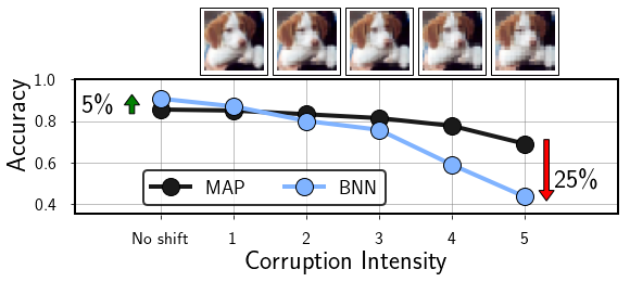
Approximate Bayesian inference for neural networks is considered a robust alternative to standard training, often providing good performance on out-of-distribution data. However, it was recently shown that Bayesian neural networks (BNNs) with high fidelity inference through Hamiltonian Monte Carlo (HMC) provide shockingly poor performance under covariate shift. For example, below we show that a ResNet-20 BNN approximated with HMC underperforms a maximum a-posteriori (MAP) solution by 25% on the pixelate-corrupted CIFAR-10 test set. This result is particularly surprising given that on the in-distribution test data, the BNN outperforms the MAP solution by over 5%. In this work, we seek to understand, further demonstrate, and help remedy this concerning behaviour.
As an example, let us consider a fully-connected network on MNIST. MNIST contains many dead pixels, i.e. pixels near the boundary that are zero for all training images. The corresponding weights in the first layer of the network are always multiplied by zero, and have no effect on the likelihood of the training data. Consequently, in a Bayesian neural network, these weights will be sampled from the prior. A MAP solution on the other hand will set these parameters close to zero. In the animation, we visualize the weights in the first layer of a Bayesian neural network and a MAP solution. For each sample, we show the value of the weight corresponding to the highlighted pixel.
If at test time the data is corrupted, e.g. by Gaussian noise, and the pixels near the boundary of the image are activated, the MAP solution will ignore these pixels, while the predictions of the BNN will be significantly affected.
In the paper, we extend this reasoning to general linear dependencies between input features for both fully connected and convolutional Bayesian neural networks. We also propose EmpCov, a prior based on the empirical covariance of the data which significantly improves robustness of BNNs to covariate shift. We implement EmpCov as well as other priors for Bayesian neural networks in this repo.
Requirements
We use provide a requirements.txt file that can be used to create a conda environment to run the code in this repo:
conda create --name <env> --file requirements.txt
Example set-up using pip:
pip install tensorflow

pip install --upgrade pip
pip install --upgrade jax jaxlib==0.1.65+cuda112 -f \
https://storage.googleapis.com/jax-releases/jax_releases.html

pip install git+https://github.com/deepmind/dm-haiku
pip install tensorflow_datasets
pip install tabulate
pip install optax
Please see the JAX repo for the latest instructions on how to install JAX on your hardware.
File Structure
The implementations of HMC and other methods forked from the BNN HMC repo are in the bnn_hmc folder. The main training scripts are run_hmc.py for HMC and run_sgd.py for SGD respectively. In the notebooks folder we show examples of how to extract the covariance matrices for EmpCov priors, and evaluate the results under various corruptions.
.
+-- bnn_hmc/
|   +-- core/
|   |   +-- hmc.py (The Hamiltonian Monte Carlo algorithm)
|   |   +-- sgmcmc.py (SGMCMC methods as optax optimizers)
|   |   +-- vi.py (Mean field variational inference)
|   +-- utils/ (Utility functions used by the training scripts)
|   |   +-- train_utils.py (The training epochs and update rules)
|   |   +-- models.py (Models used in the experiments)
|   |   +-- losses.py (Prior and likelihood functions)
|   |   +-- data_utils.py (Loading and pre-processing the data)
|   |   +-- optim_utils.py (Optimizers and learning rate schedules)
|   |   +-- ensemble_utils.py (Implementation of ensembling of predictions)
|   |   +-- metrics.py (Metrics used in evaluation)
|   |   +-- cmd_args_utils.py (Common command line arguments)
|   |   +-- script_utils.py (Common functionality of the training scripts)
|   |   +-- checkpoint_utils.py (Saving and loading checkpoints)
|   |   +-- logging_utils.py (Utilities for logging printing the results)
|   |   +-- precision_utils.py (Controlling the numerical precision)
|   |   +-- tree_utils.py (Common operations on pytree objects)
+-- notebooks/
|   +-- cnn_robustness_cifar10.ipynb (Creates CIFAR-10 CNN figures used in paper)
|   +-- mlp_robustness_mnist.ipynb (Creates MNIST MLP figures used in paper)
|   +-- cifar10_cnn_extract_empcov.ipynb (Constructs EmpCov prior covariance matrix for CIFAR-10 CNN)
|   +-- mnist_extract_empcov.ipynb (Constructs EmpCov prior covariance matrices for CIFAR-10 CNN and MLP)
+-- empcov_covs/
|   +-- cifar_cnn_pca_inv_cov.npy (EmpCov inverse prior covariance for CIFAR-10 CNN)
|   +-- mnist_cnn_pca_inv_cov.npy (EmpCov inverse prior covariance for MNIST CNN)
|   +-- mnist_mlp_pca_inv_cov.npy (EmpCov inverse prior covariance for MNIST MLP)
+-- run_hmc.py (HMC training script)
+-- run_sgd.py (SGD training script)
Training Scripts
The training scripts are adapted from the Google Research BNN HMC repo. For completeness, we provide full details about the command line arguments here.
Common command line arguments:
seed— random seeddir— training directory for saving the checkpoints and tensorboard logsdataset_name— name of the dataset, e.g.cifar10,cifar100,mnistsubset_train_to— number of datapoints to use from the dataset; by default, the full dataset is usedmodel_name— name of the neural network architecture, e.g.lenet,resnet20_frn_swish,cnn_lstm,mlp_regression_smallweight_decay— weight decay; for Bayesian methods, weight decay determines the prior variance (prior_var = 1 / weight_decay)temperature— posterior temperature (default:1)init_checkpoint— path to the checkpoint to use for initialization (optional)tabulate_freq— frequency of tabulate table header logginguse_float64— use float64 precision (does not work on TPUs and some GPUs); by default, we usefloat32precisionprior_family— type of prior to use; must be one ofGaussian,ExpFNormP,Laplace,StudentT,SumFilterLeNet,EmpCovLeNetorEmpCovMLP; see the next section for more details
Prior Families
In this repo we implement several prior distribution families. Some of the prior families have additional command line arguments specifying the parameters of the prior:
Gaussian— iid Gaussian prior centered at0with variance equal to1 / weight_decayLaplace— iid Laplace prior centered at0with variance equal to1 / weight_decayStudentT— iid Laplace prior centered at0withstudentt_degrees_of_freedomdegrees of freedom and scaled by1 / weight_decayExpFNormP— iid ExpNorm prior centered at0defined in the paper.expfnormp_powerspecifies the power under the exponent in the prior, and1 / weight_decaydefines the scale of the priorEmpCovLeNetandEmpCovMLP— EmpCov priors with the inverse of empirical covariance matrix of the data as a.npyarray provided asempcov_invcov_ckpt;empcov_wdallows to rescale the covariance matrix for the first layer.SumFilterLeNet— SumFilter prior presented in the paper;1 / sumfilterlenet_weight_decaydetermines the prior variance for the sum of the filter weights in the first layer
Some prior types require additional arguments, such as empcov_pca_wd and studentt_degrees_of_freedom; run scripts with --help for full details.
Running HMC
To run HMC, you can use the run_hmc.py training script. Arguments:
step_size— HMC step sizetrajectory_len— HMC trajectory lengthnum_iterations— Total number of HMC iterationsmax_num_leapfrog_steps— Maximum number of leapfrog steps allowed; meant as a sanity check and should be greater thantrajectory_len / step_sizenum_burn_in_iterations— Number of burn-in iterations (default:0)
Examples
CNN on CIFAR-10 with different priors:
# Gaussian prior
python3 run_hmc.py --seed=0 --weight_decay=100 --temperature=1. \
  --dir=runs/hmc/cifar10/gaussian/ --dataset_name=cifar10 \
  --model_name=lenet --step_size=3.e-05 --trajectory_len=0.15 \
  --num_iterations=100 --max_num_leapfrog_steps=5300 \
  --num_burn_in_iterations=10

# Laplace prior
python3 run_hmc.py --seed=0 --weight_decay=100 --temperature=1. \
  --dir=runs/hmc/cifar10/laplace --dataset_name=cifar10 \
  --model_name=lenet --step_size=3.e-05 --trajectory_len=0.15 \
  --num_iterations=100 --max_num_leapfrog_steps=5300 \
  --num_burn_in_iterations=10 --prior_family=Laplace

# Gaussian prior, T=0.1
python3  run_hmc.py --seed=0 --weight_decay=3 --temperature=0.01 \
  --dir=runs/hmc/cifar10/lenet/temp --dataset_name=cifar10 \
  --model_name=lenet --step_size=1.e-05 --trajectory_len=0.1 \
  --num_iterations=100 --max_num_leapfrog_steps=10000 \
  --num_burn_in_iterations=10

# EmpCov prior
python3 run_hmc.py --seed=0 --weight_decay=100. --temperature=1. \
  --dir=runs/hmc/cifar10/EmpCov --dataset_name=cifar10 \
  --model_name=lenet --step_size=1.e-4 --trajectory_len=0.157 \
  --num_iterations=100 --max_num_leapfrog_steps=2000 \
  --num_burn_in_iterations=10 --prior_family=EmpCovLeNet \
  --empcov_invcov_ckpt=empcov_covs/cifar_cnn_pca_inv_cov.npy \
  --empcov_wd=100.
We ran these commands on a machine with 8 NVIDIA Tesla V-100 GPUs.
MLP on MNIST using different priors:
# Gaussian prior
python3 run_hmc.py --seed=2 --weight_decay=100  \
  --dir=runs/hmc/mnist/gaussian \
  --dataset_name=mnist --model_name=mlp_classification \
  --step_size=1.e-05 --trajectory_len=0.15 \
  --num_iterations=100 --max_num_leapfrog_steps=15500 \
  --num_burn_in_iterations=10

# Laplace prior
python3 run_hmc.py --seed=0 --weight_decay=3.0 \
  --dir=runs/hmc/mnist/laplace --dataset_name=mnist \
  --model_name=mlp_classification --step_size=6.e-05 \
  --trajectory_len=0.9 --num_iterations=100 \
  --max_num_leapfrog_steps=15500 \
  --num_burn_in_iterations=10 --prior_family=Laplace

# Student-T prior
python3 run_hmc.py --seed=0 --weight_decay=10. \
  --dir=runs/hmc/mnist/studentt --dataset_name=mnist \
  --model_name=mlp_classification --step_size=1.e-4 --trajectory_len=0.49 \
  --num_iterations=100 --max_num_leapfrog_steps=5000 \
  --num_burn_in_iterations=10 --prior_family=StudentT \
  --studentt_degrees_of_freedom=5.

# Gaussian prior, T=0.1
python3 run_hmc.py --seed=11 --weight_decay=100 \
  --temperature=0.01 --dir=runs/hmc/mnist/temp \
  --dataset_name=mnist --model_name=mlp_classification \
  --step_size=6.3e-07 --trajectory_len=0.015 \
  --num_iterations=100 --max_num_leapfrog_steps=25500 \
  --num_burn_in_iterations=10

# EmpCov prior
python3 run_hmc.py --seed=0 --weight_decay=100 \
  --dir=runs/hmc/mnist/empcov --dataset_name=mnist \
  --model_name=mlp_classification --step_size=1.e-05 \
  --trajectory_len=0.15 --num_iterations=100 \
  --max_num_leapfrog_steps=15500 \
  --num_burn_in_iterations=10 --prior_family=EmpCovMLP \
  --empcov_invcov_ckpt=empcov_covs/mnist_mlp_pca_inv_cov.npy \
  --empcov_wd=100
This script can be ran on a single GPU or a TPU V3-8.
Running SGD
To run SGD, you can use the run_sgd.py training script. Arguments:
init_step_size— Initial SGD step size; we use a cosine schedulenum_epochs— total number of SGD epochs iterationsbatch_size— batch sizeeval_freq— frequency of evaluation (epochs)save_freq— frequency of checkpointing (epochs)momentum_decay— momentum decay parameter for SGD
Examples
MLP on MNIST:
python3 run_sgd.py --seed=0 --weight_decay=100 --dir=runs/sgd/mnist/ \
  --dataset_name=mnist --model_name=mlp_classification \
  --init_step_size=1e-7 --eval_freq=10 --batch_size=80 \
  --num_epochs=100 --save_freq=100
CNN on CIFAR-10:
python3 run_sgd.py --seed=0 --weight_decay=100. --dir=runs/sgd/cifar10/lenet \
  --dataset_name=cifar10 --model_name=lenet --init_step_size=1e-7 --batch_size=80 \
  --num_epochs=300 --save_freq=300
To train a deep ensemble, we simply train multiple copies of SGD with different random seeds.
Results
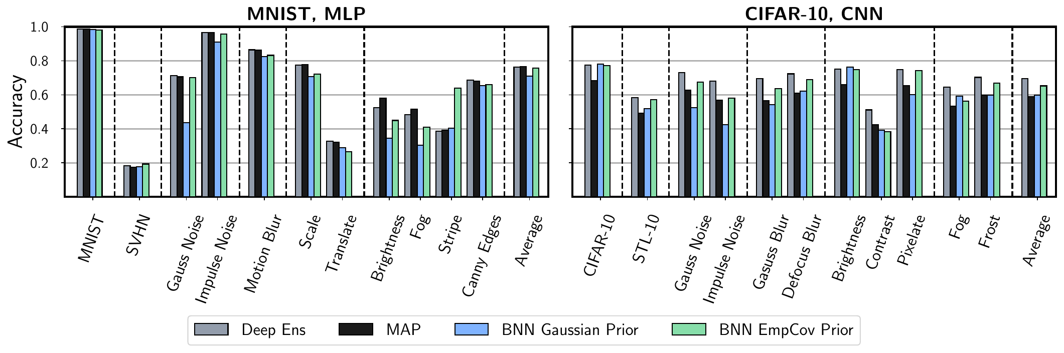
We consider the corrupted versions of the MNIST and CIFAR-10 datasets with both fully-connected (mlp_classification) and convolutional (lenet) architectures. Additionally, we consider domain shift problems from MNIST to SVHN and from CIFAR-10 to STL-10. We apply the EmpCov prior to the first layer of Bayesian neural networks (BNNs), and a Gaussian prior to all other layers using the commands in the examples. The following figure shows the results for: deep ensembles, maximum-a-posterior estimate obtained through SGD, BNNs with a Gaussian prior, and BNNs with our novel EmpCov prior. EmpCov prior improves the robustness of BNNs to covariate shift, leading to better results on most corruptions and a competitive performance with deep ensembles for both fully-connected and convolutional architectures.