skggm

In the last decade, learning networks that encode conditional independence relationships has become an important problem in machine learning and statistics. For many important probability distributions, such as multivariate Gaussians, this amounts to estimation of inverse covariance matrices. Inverse covariance estimation is now used widely in infer gene regulatory networks in cellular biology and neural interactions in the neuroscience.

However, many statistical advances and best practices in fitting such models to data are not yet widely adopted and not available in common python packages for machine learning. Furthermore, inverse covariance estimation is an active area of research where researchers continue to improve algorithms and estimators.
With skggm we seek to provide these new developments to a wider audience, and also enable researchers to effectively benchmark their methods in regimes relevant to their applications of interest.

While skggm is currently geared toward Gaussian graphical models, we hope to eventually evolve it to support General graphical models. Read more here.

Inverse Covariance Estimation

Given n independently drawn, p-dimensional Gaussian random samples with sample covariance , the maximum likelihood estimate of the inverse covariance matrix $\lambda$ can be computed via the graphical lasso, i.e., the program

$\ell_1 penalized inverse covariance estimation$

where $\Lambda$ is a symmetric matrix with non-negative entries and

penalty

Typically, the diagonals are not penalized by setting to ensure that Theta remains positive definite. The objective reduces to the standard graphical lasso formulation of Friedman et al. when all off diagonals of the penalty matrix take a constant scalar value scalar_penalty . The standard graphical lasso has been implemented in scikit-learn.

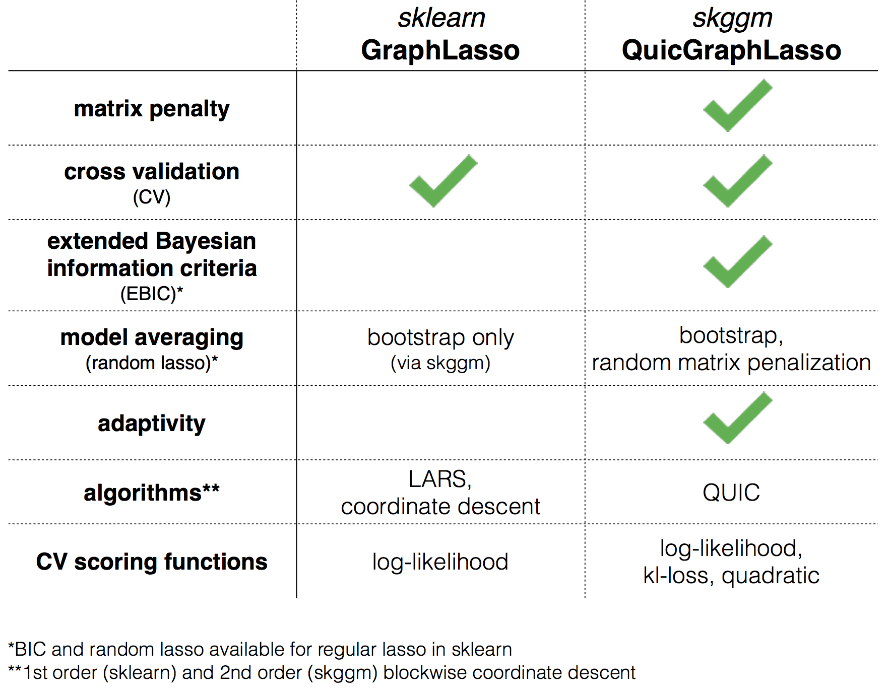
In this package we provide a scikit-learn-compatible implementation of the program above and a collection of modern best practices for working with the graphical lasso. A rough breakdown of how this package differs from scikit's built-in GraphLasso is depicted by this chart:

sklearn/skggm feature comparison

Quick start

To get started, install the package (via pip, see below) and:

read the tour of skggm at https://skggm.github.io/skggm/tour
read @mnarayan's talk and check out the companion examples here (live via binder at here). Presented at HHMI, Janelia Farms, October 2016.
basic usage examples can be found in examples/estimator_suite.py

This is an ongoing effort. We'd love your feedback on which algorithms and techniques we should include and how you're using the package. We also welcome contributions.

@jasonlaska and @mnarayan

Included in `inverse_covariance`

An overview of the skggm graphical lasso facilities is depicted by the following diagram:

sklearn/skggm feature comparison

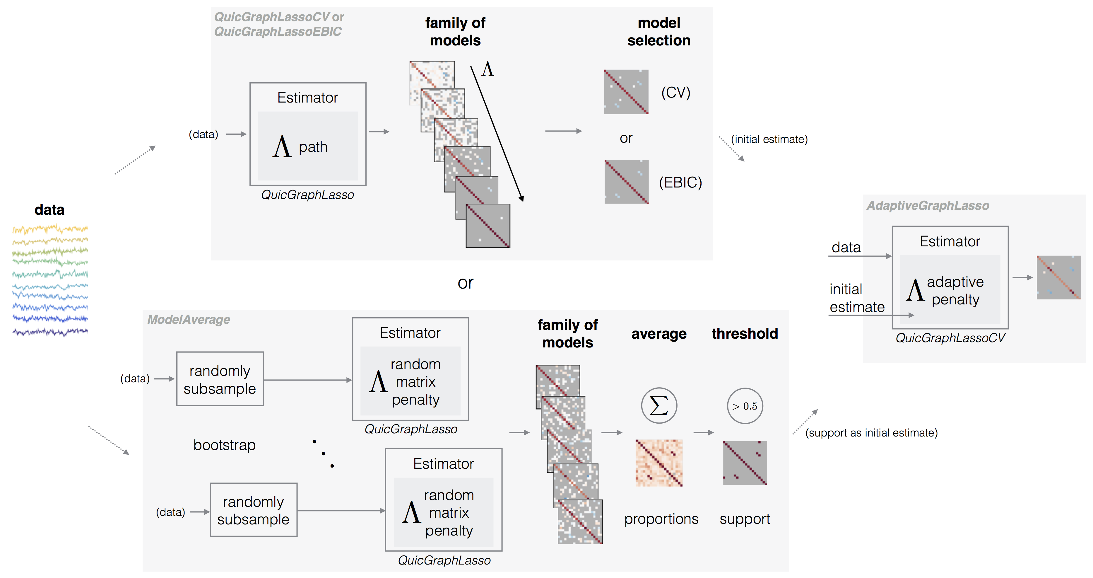
Information on basic usage can be found at https://skggm.github.io/skggm/tour. The package includes the following classes and submodules.

QuicGraphicalLasso [doc]

QuicGraphicalLasso is an implementation of QUIC wrapped as a scikit-learn compatible estimator [Hsieh et al.] . The estimator can be run in default mode for a fixed penalty or in path mode to explore a sequence of penalties efficiently. The penalty lam can be a scalar or matrix.

The primary outputs of interest are: covariance_, precision_, and lam_.

The interface largely mirrors the built-in GraphLasso although some param names have been changed (e.g., alpha to lam). Some notable advantages of this implementation over GraphicalLasso are support for a matrix penalization term and speed.
QuicGraphicalLassoCV [doc]

QuicGraphicalLassoCV is an optimized cross-validation model selection implementation similar to scikit-learn's GraphLassoCV. As with QuicGraphicalLasso, this implementation also supports matrix penalization.
QuicGraphicalLassoEBIC [doc]

QuicGraphicalLassoEBIC is provided as a convenience class to use the Extended Bayesian Information Criteria (EBIC) for model selection [Foygel et al.].
ModelAverage [doc]

ModelAverage is an ensemble meta-estimator that computes several fits with a user-specified estimator and averages the support of the resulting precision estimates. The result is a proportion_ matrix indicating the sample probability of a non-zero at each index. This is a similar facility to scikit-learn's RandomizedLasso) but for the graph lasso.

In each trial, this class will:
1. Draw bootstrap samples by randomly subsampling X.
2. Draw a random matrix penalty.
The random penalty can be chosen in a variety of ways, specified by the penalization parameter. This technique is also known as stability selection or random lasso.
AdaptiveGraphicalLasso [doc]

AdaptiveGraphicalLasso performs a two step estimation procedure:
1. Obtain an initial sparse estimate.
2. Derive a new penalization matrix from the original estimate. We currently provide three methods for this: binary, 1/|coeffs|, and 1/|coeffs|^2. The binary method only requires the initial estimate's support (and this can be be used with ModelAverage below).
This technique works well to refine the non-zero precision values given a reasonable initial support estimate.
inverse_covariance.plot_util.trace_plot

Utility to plot lam_ paths.
inverse_covariance.profiling

The .profiling submodule contains a MonteCarloProfiling() class for evaluating methods over different graphs and metrics. We currently include the following graph types:
```
  - LatticeGraph
  - ClusterGraph
  - ErdosRenyiGraph (via sklearn)
```
An example of how to use these tools can be found in examples/profiling_example.py.

Parallelization Support

skggm supports parallel computation through joblib and Apache Spark. Independent trials, cross validation, and other embarrassingly parallel operations can be farmed out to multiple processes, cores, or worker machines. In particular,

QuicGraphicalLassoCV
ModelAverage
profiling.MonteCarloProfile

can make use of this through either the n_jobs or sc (sparkContext) parameters.

Since these are naive implementations, it is not possible to enable parallel work on all three of objects simultaneously when they are being composited together. For example, in this snippet:

model = ModelAverage(
    estimator=QuicGraphicalLassoCV(
        cv=2,
        n_refinements=6,
    )
    penalization=penalization,
    lam=lam,
    sc=spark.sparkContext,
)
model.fit(X)

only one of ModelAverage or QuicGraphicalLassoCV can make use of the spark context. The problem size and number of trials will determine the resolution that gives the fastest performance.

Installation

Both python2.7 and python3.6.x are supported. We use the black autoformatter to format our code. If contributing, please run this formatter checks will fail.

Clone this repo and run

python setup.py install

or via PyPI

pip install skggm

or from a cloned repo

cd inverse_covariance/pyquic
make
make python3  (for python3)

The package requires that numpy, scipy, and cython are installed independently into your environment first.

If you would like to fork the pyquic bindings directly, use the Makefile provided in inverse_covariance/pyquic.

This package requires the lapack libraries to by installed on your system. A configuration example with these dependencies for Ubuntu and Anaconda 2 can be found here.

Tests

To run the tests, execute the following lines.

python -m pytest inverse_covariance (python3 -m pytest inverse_covariance)
black --check inverse_covariance
black --check examples

Examples

Usage

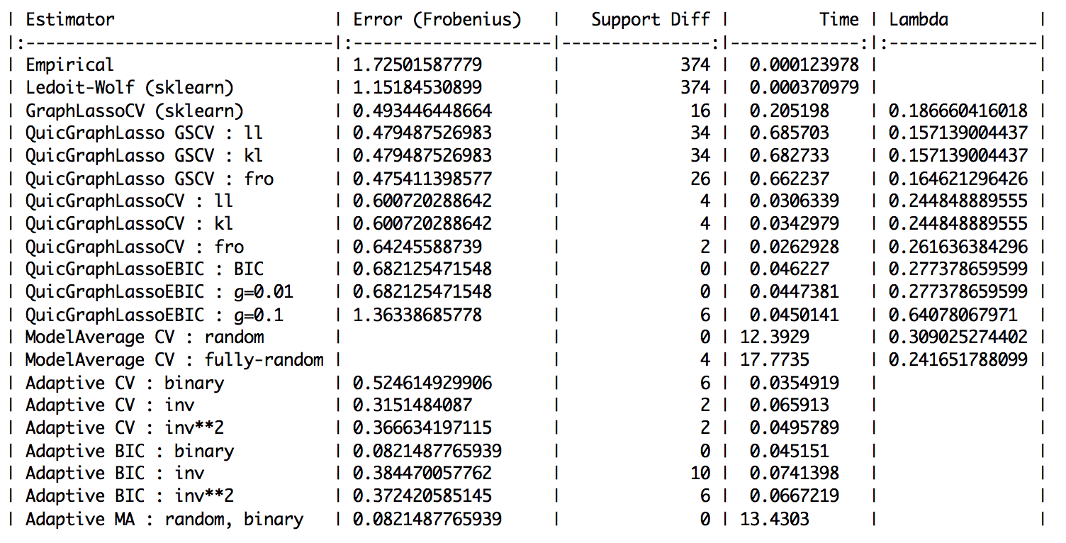
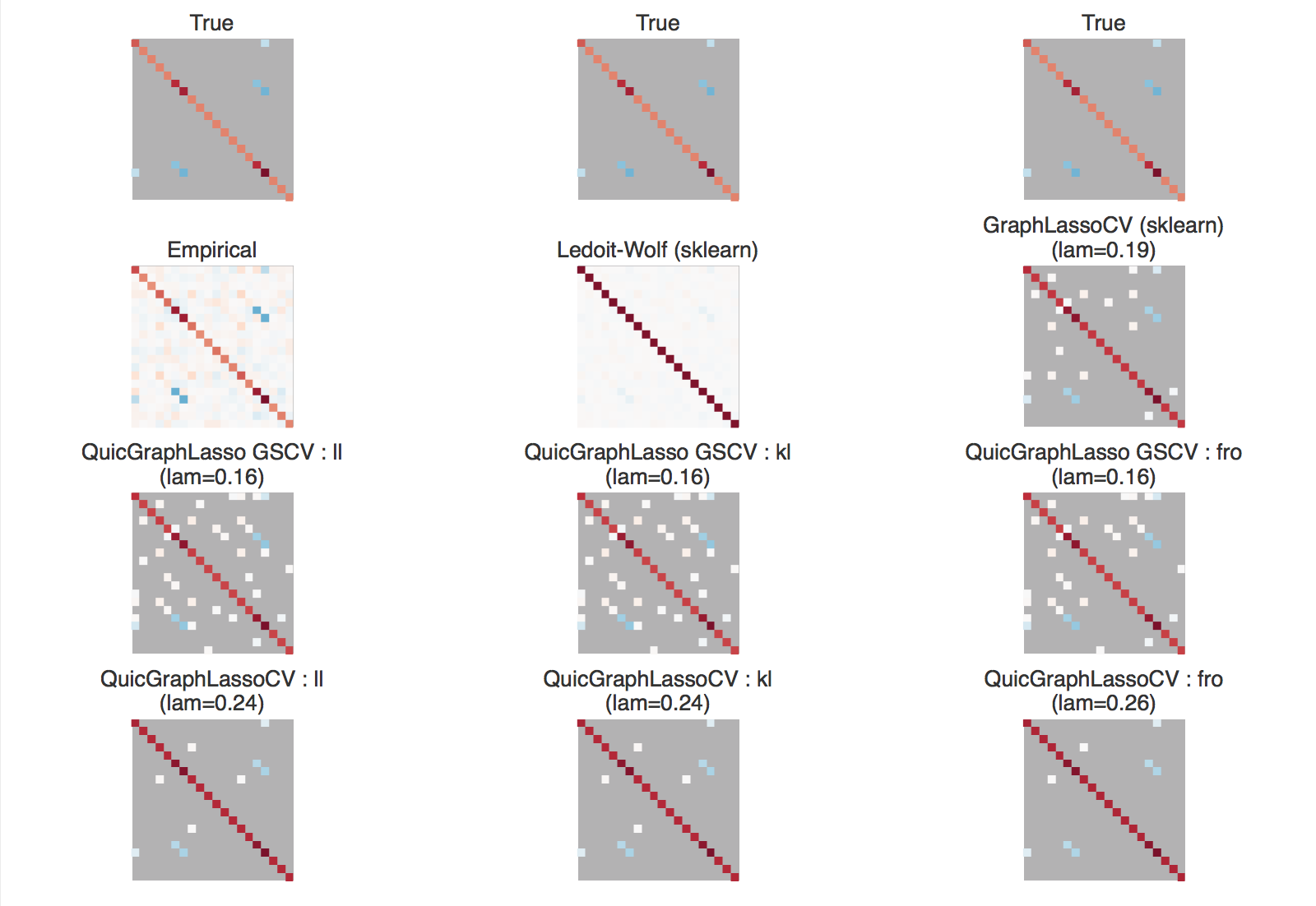
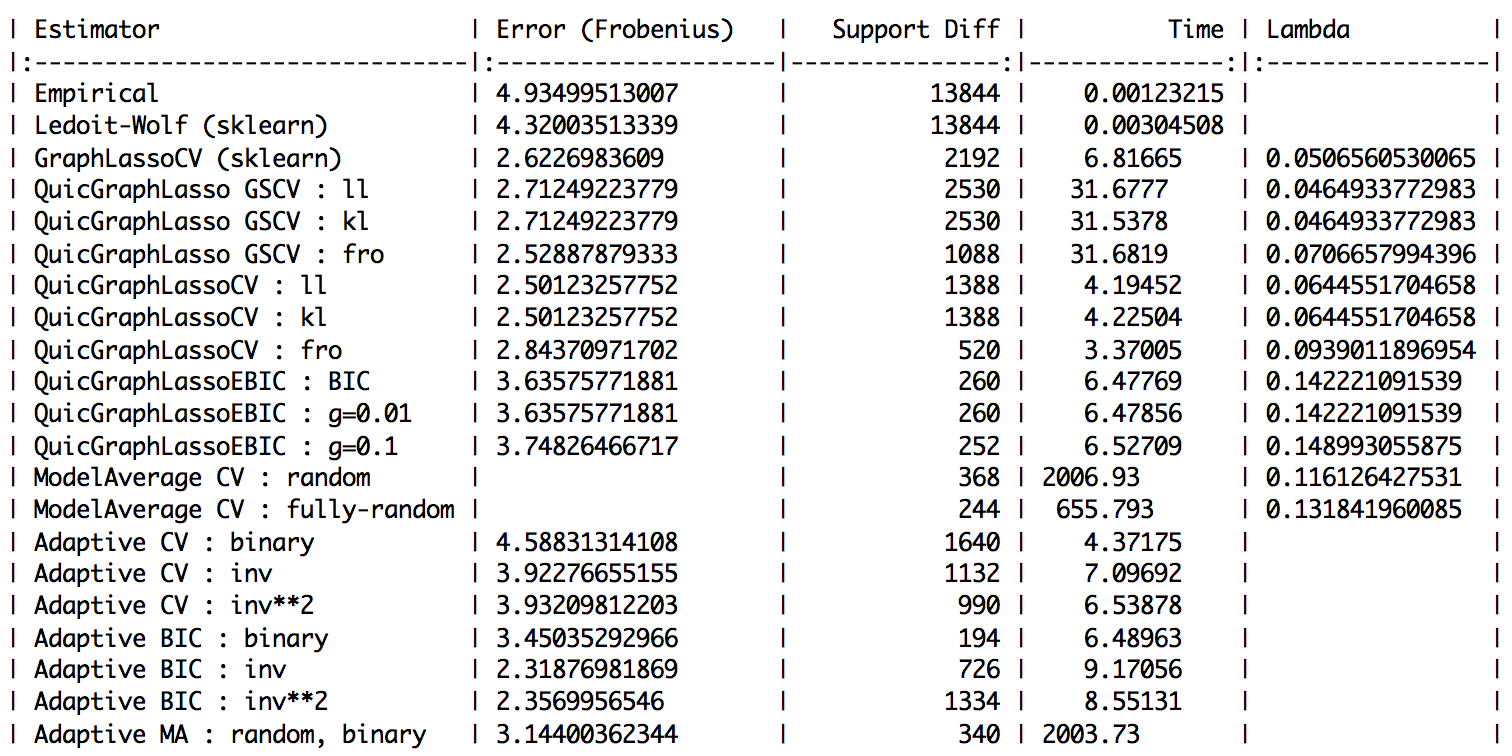
In examples/estimator_suite.py we reproduce the plot_sparse_cov example from the scikit-learn documentation for each method provided (however, the variations chosen are not exhaustive).

An example run for n_examples=100 and n_features=20 yielded the following results.

(n_examples, n_features) = (100, 20)

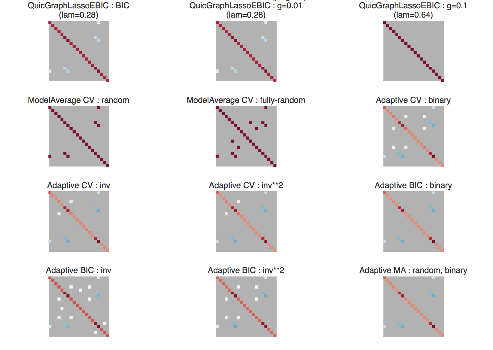
For slightly higher dimensions of n_examples=600 and n_features=120 we obtained:

(n_examples, n_features) = (600, 120)

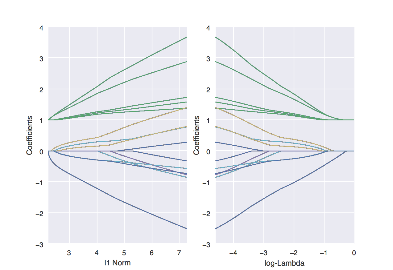
Plotting the regularization path

We've provided a utility function inverse_covariance.plot_util.trace_plot that can be used to display the coefficients as a function of lam_. This can be used with any estimator that returns a path. The example in examples/trace_plot_example.py yields:

Trace plot

Citation

If you use skggm or reference our blog post in a presentation or publication, we would appreciate citations of our package.

Jason Laska, Manjari Narayan, 2017. skggm 0.2.7: A scikit-learn compatible package for Gaussian and related Graphical Models. doi:10.5281/zenodo.830033

Here is the corresponding Bibtex entry

@misc{laska_narayan_2017_830033,
  author       = {Jason Laska and
                  Manjari Narayan},
  title        = {{skggm 0.2.7: A scikit-learn compatible package for
                   Gaussian and related Graphical Models}},
  month        = jul,
  year         = 2017,
  doi          = {10.5281/zenodo.830033},
  url          = {https://doi.org/10.5281/zenodo.830033}
}