Minimisation of a negative log likelihood fit to extract the lifetime of the D^0 meson (MNLL2ELDM)
Introduction
The average lifetime of the $D^{0}$ mesons was computed from 10,000 experimental data of the decay time and the associated error by minimising the negative log-likelihood (NLL) corresponding to cases with and without the background signals. In the absence of possible background signals, the parabolic minimisation method was employed, yielding the average lifetime as $(404.5 +/- 4.7) x 10^-15 seconds with a tolerance level of 10^-6. This result was found to be inconsistent with the literature value provided by the Particle Data Group, showing a deviation of approximately 6 x 10^-15 seconds. By considering possible background signals, an alternative distribution and the corresponding NLL were derived. This was subsequently minimised using the gradient, Newton’s and the Quasi-Newton methods, yielding consistent results. The average lifetime and the fraction of the background signals in the sample were estimated to be (409.7 +/- 5.5) x 10^-15 seconds and 0.0163 +/- .0086$, respectively, where the uncertainties were calculated using an error matrix and the correlation coefficient was found to be -0.4813. The literature value lies within the uncertainty, showing a percentage difference of approximately 0.098%. Thus the results verify the presence of the background signals in the data and validate the theory of the expected distribution derived by assuming the background signal as a Gaussian due the limitation of the detector resolution.
Requirements
Python 2.x is required to run the script
Create an environment using conda as follows:
conda create -n python2 python=2.x
Then activate the new environment by:
conda activate python2
Results
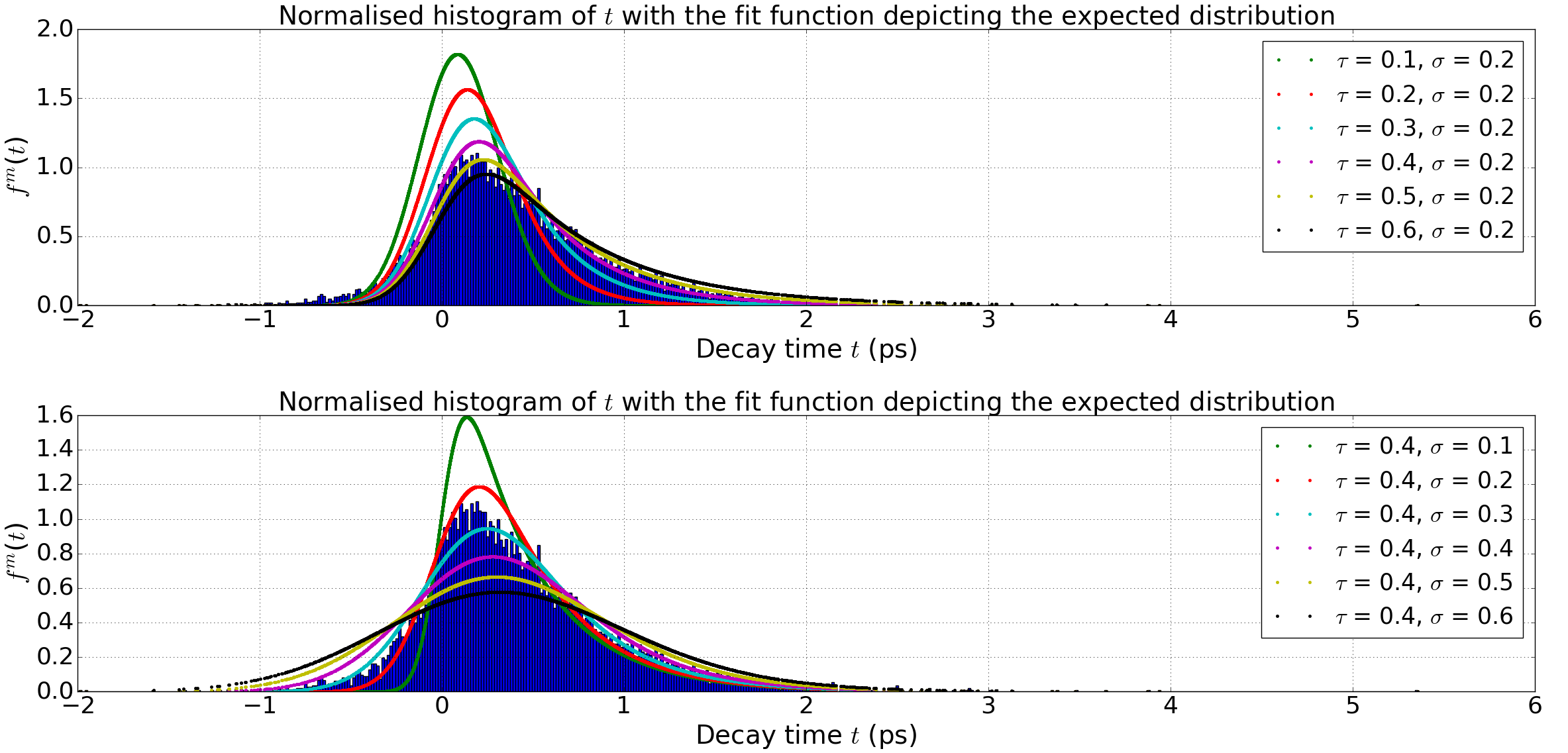
Figure 1: Histogram of the measured decay time of D^0 mesons and the expected distribution with various tau and sigma in the units of picoseconds. The figure illustrates that the average lifetime is approximately between 0.4 ps and 0.5 ps, being closer to the former value. The second figure clearly demonstrates that the distribution with tau = 0.4 ps and sigma = 0.2 ps fits the profile of the histogram the most closest.
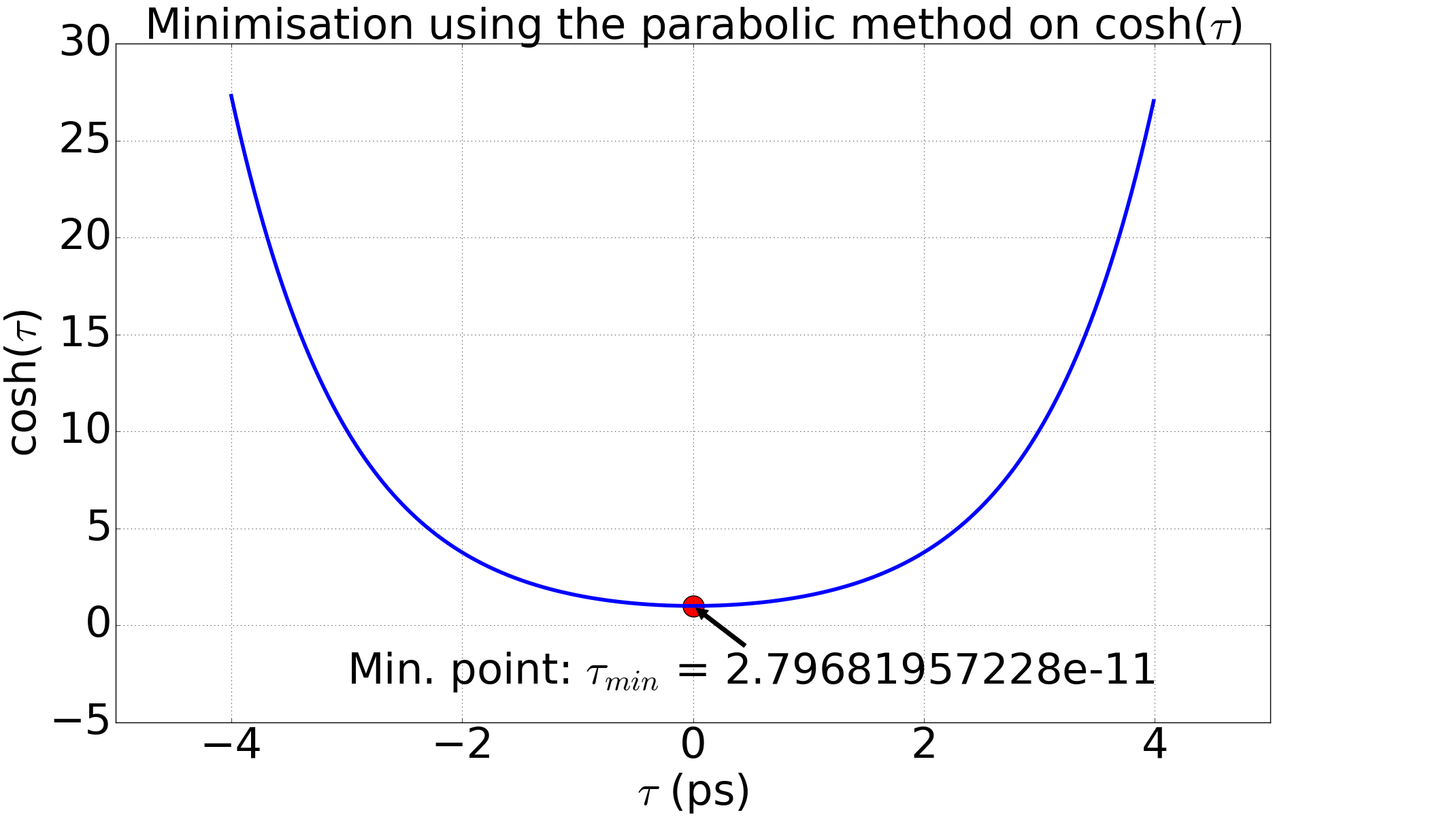
Figure 2: Result of the minimisation using the parabolic method on a hyperbolic cosine function. The initial guesses were 2 ps, 3 ps and 5 ps, and the minimum is estimated to be at tau = 2.80 x 10^-11 (3 s.f.) using a tolerance level of 10^-6.
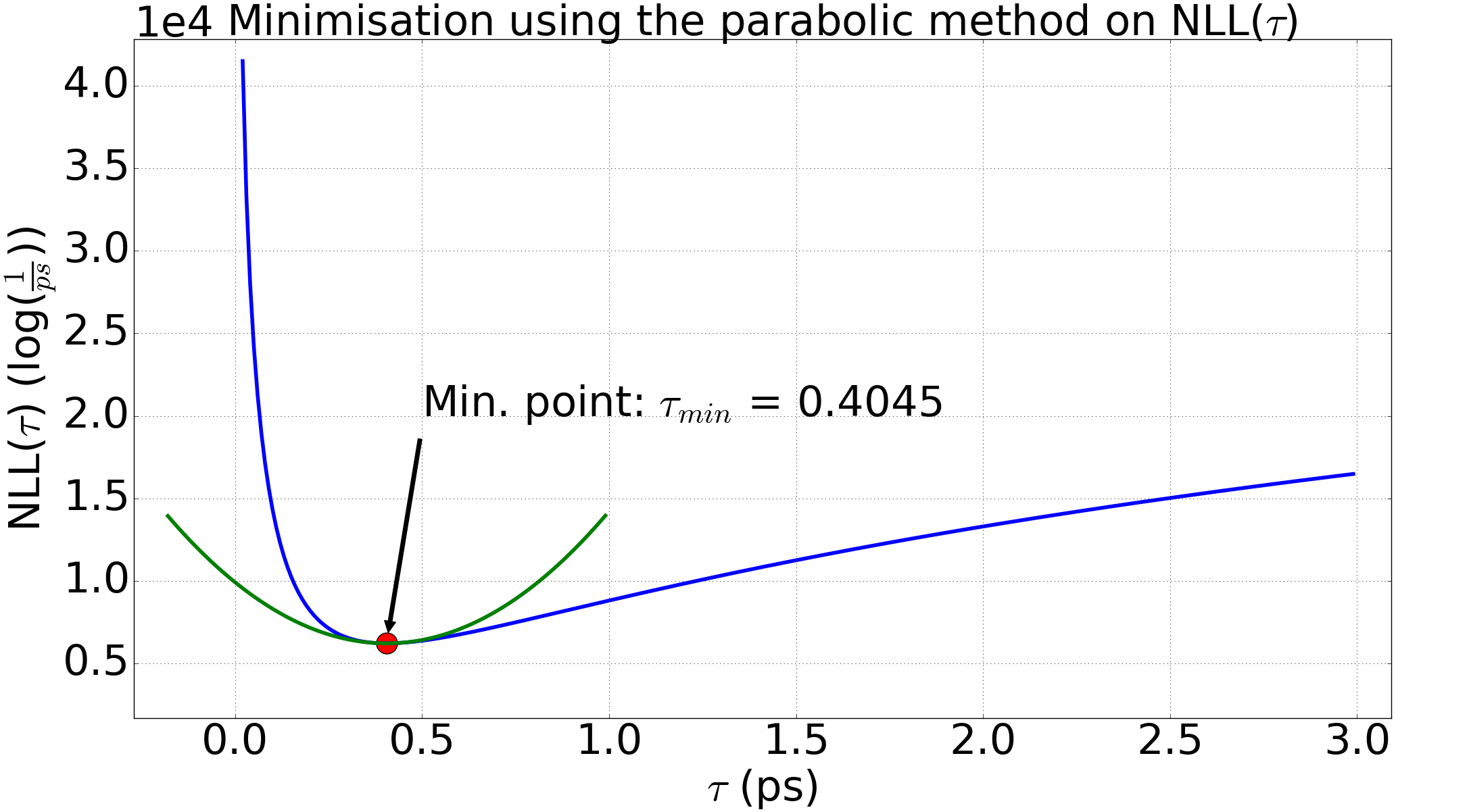
Figure 3: Graph of the 1-D NLL. The minimisation yielded the minimum as tau_min = 0.4045 ps correct to 4 d.p. with a tolerance level of 10^-6. The minimum was originally estima- ted to be roughly 0.40 ps, which is equal to the result correct to 2 d.p. Moreover, the parabola with a curvature of 22,572 illustrates its suitability in approximating the minimum.
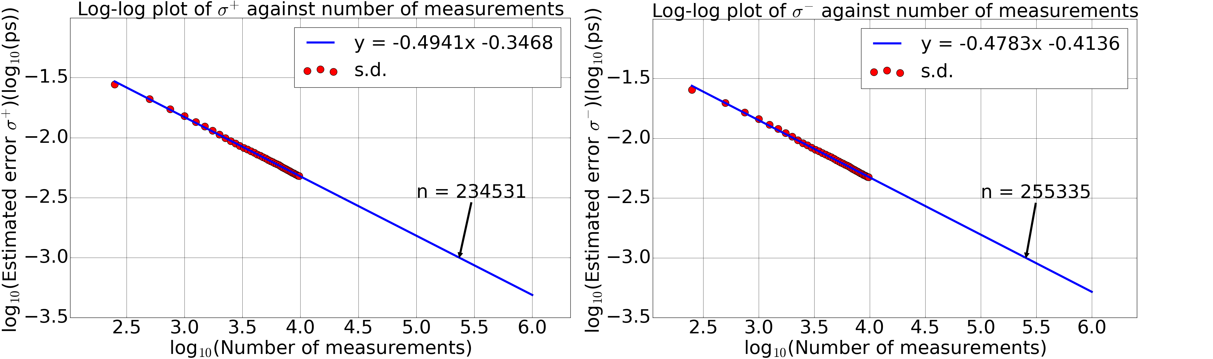
Figure 4: The dependence of the standard deviation on the number of measurements in logarithmic scales. The minimisation of NLL function took initial guesses of 0.2 ps, 0.3 ps and 0.5 ps. Each figure depicts a linearly decreasing pattern of the standard deviation with the number of measurements in logarithmic scales. Thus a linear fit was applied and it was extrapolated, assuming the pattern stayed linear in the region of interest. The extrapolation yielded the required number of measurements for an accuracy of 10^-15 s as (2.3 to 2.6) x 10^5.

Figure 5: Contour plots of the 2D hyperbolic cosine function showing the result from the minimisation with an initial condition of (x, y) = (-2.5, 3.0), step-length of alpha = 0.05 and a tolerance level of 10^-6. The left figure is an enlarged version of the right. The minimum estimated using the Quasi-Newton, gradient and Newton’s methods are: (x, y) = (-1.92, 1.91) x 10^-5, (x, y) = (-1.86, 1.96) x 10^-5 and (x, y) = (-2.42 x 10^-13, 6.72 x 10^-8} with 213, 222 and 5 iterations, respectively. The results graphically demonstrate the minimisation process with all the methods yielding expected results and thus confirming the validity of the computation. The paths generated by the Quasi-Newton and the gradient methods show only a small difference with similar number of iterations, whereas Newton’s method illustrates a greater converging speed.
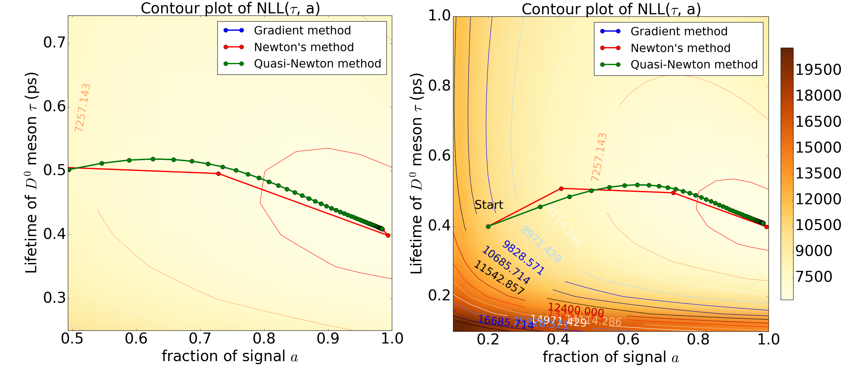
Figure 6: Contour plots of the 2D NLL function showing the result from the minimisation with initial condition of (a, tau) = (0.2, 0.4 ps), step-length of alpha = 0.00001 and a tolerance level of 10^-6. The plot of the left is an enlarged version of the plot on the right. The positions of the minimum estimated using the Quasi-Newton, gradient and Newton’s methods were identical correct to 4 d.p. The estimated position of the minimum is (a, tau) = (0.9837, 0.4097 ps) with 98 iterations for the first two methods and 6 for the third. The figures show that the paths taken during the minimisation process are almost identical for the Quasi-Newton and the gradient method; the blue curve virtually superimposes the green curve. The path generated by Newton’s method, on the other hand, differs and identifies the minimum in relatively small number of iterations. Note: CDS was used to approximate the gradients for this particular result.
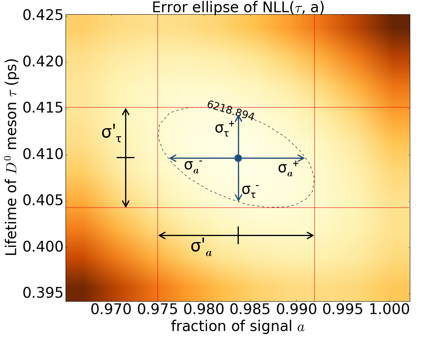
Figure 7: The error ellipse – a contour plot corresponding to one standard deviation change in the parameters above the minimum.