Most popular metrics used to evaluate object detection algorithms

Metrics for object detection

The motivation of this project is the lack of consensus used by different works and implementations concerning the evaluation metrics of the object detection problem. Although on-line competitions use their own metrics to evaluate the task of object detection, just some of them offer reference code snippets to calculate the accuracy of the detected objects.
Researchers who want to evaluate their work using different datasets than those offered by the competitions, need to implement their own version of the metrics. Sometimes a wrong or different implementation can create different and biased results. Ideally, in order to have trustworthy benchmarking among different approaches, it is necessary to have a flexible implementation that can be used by everyone regardless the dataset used.

This project provides easy-to-use functions implementing the same metrics used by the the most popular competitions of object detection. Our implementation does not require modifications of your detection model to complicated input formats, avoiding conversions to XML or JSON files. We simplified the input data (ground truth bounding boxes and detected bounding boxes) and gathered in a single project the main metrics used by the academia and challenges. Our implementation was carefully compared against the official implementations and our results are exactly the same.

In the topics below you can find an overview of the most popular metrics used in different competitions and works, as well as samples showing how to use our code.

Important definitions

Intersection Over Union (IOU)

Intersection Over Union (IOU) is measure based on Jaccard Index that evaluates the overlap between two bounding boxes. It requires a ground truth bounding box and a predicted bounding box . By applying the IOU we can tell if a detection is valid (True Positive) or not (False Positive).
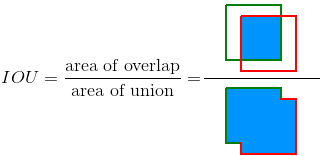
IOU is given by the overlapping area between the predicted bounding box and the ground truth bounding box divided by the area of union between them:

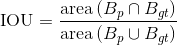
The image below illustrates the IOU between a ground truth bounding box (in green) and a detected bounding box (in red).

True Positive, False Positive, False Negative and True Negative

Some basic concepts used by the metrics:

• True Positive (TP): A correct detection. Detection with IOU ≥ threshold
• False Positive (FP): A wrong detection. Detection with IOU < threshold
• False Negative (FN): A ground truth not detected
• True Negative (TN): Does not apply. It would represent a corrected misdetection. In the object detection task there are many possible bounding boxes that should not be detected within an image. Thus, TN would be all possible bounding boxes that were corrrectly not detected (so many possible boxes within an image). That's why it is not used by the metrics.

threshold: depending on the metric, it is usually set to 50%, 75% or 95%.

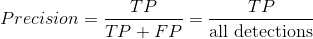
Precision

Precision is the ability of a model to identify only the relevant objects. It is the percentage of correct positive predictions and is given by:

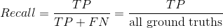
Recall

Recall is the ability of a model to find all the relevant cases (all ground truth bounding boxes). It is the percentage of true positive detected among all relevant ground truths and is given by:

Metrics

In the topics below there are some comments on the most popular metrics used for object detection.

Precision x Recall curve

The Precision x Recall curve is a good way to evaluate the performance of an object detector as the confidence is changed. There is a curve for each object class. An object detector of a particular class is considered good if its prediction stays high as recall increases, which means that if you vary the confidence threshold, the precision and recall will still be high. Another way to identify a good object detector is to look for a detector that can identify only relevant objects (0 False Positives = high precision), finding all ground truth objects (0 False Negatives = high recall).

A poor object detector needs to increase the number of detected objects (increasing False Positives = lower precision) in order to retrieve all ground truth objects (high recall). That's why the Precision x Recall curve usually starts with high precision values, decreasing as recall increases. You can see an example of the Prevision x Recall curve in the next topic (Average Precision).
This kind of curve is used by the PASCAL VOC 2012 challenge and is available in our implementation.

Average Precision

Another way to compare the performance of object detectors is to calculate the area under the curve (AUC) of the Precision x Recall curve. As AP curves are often zigzag curves frequently going up and down, comparing different curves (different detectors) in the same plot usually is not an easy task - because the curves tend to cross each other much frequently. That's why Average Precision (AP), a numerical metric, can also help us compare different detectors. In practice AP is the precision averaged across all recall values between 0 and 1.

PASCAL VOC 2012 challenge uses the interpolated average precision. It tries to summarize the shape of the Precision x Recall curve by averaging the precision at a set of eleven equally spaced recall levels [0, 0.1, 0.2, ... , 1]:

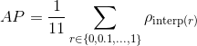
with

where is the measured precision at recall .

Instead of using the precision observed at each point, the AP is obtained by interpolating the precision at each level taking the maximum precision whose recall value is greater than .

An ilustrated example

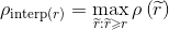
An example helps us understand better the concept of the interpolated average precision. Consider the detections below:

There are 7 images with 15 ground truth objects representented by the green bounding boxes and 24 detected objects represented by the red bounding boxes. Each detected object has a confidence level and is identified by a letter (A,B,...,Y).

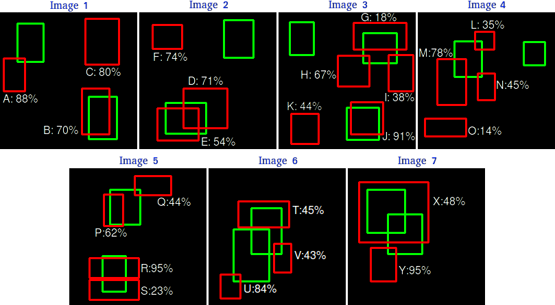
The following table shows the bounding boxes with their corresponding confidences. The last column identifies the detections as TP or FP. In this example a TP is considered if IOU 30%, otherwise it is a FP. By looking at the images above we can roughly tell if the detections are TP or FP.

In some images there are more than one detection overlapping a ground truth (Images 2, 3, 4, 5, 6 and 7). For those cases the detection with the highest IOU is taken, discarding the other detections. This rule is applied by the PASCAL VOC 2012 metric: "e.g. 5 detections (TP) of a single object is counted as 1 correct detection and 4 false detections”.

The Precision x Recall curve is plotted by calculating the precision and recall values of the accumulated TP or FP detections. For this, first we need to order the detections by their confidences, then we calculate the precision and recall for each accumulated detection as shown in the table below:

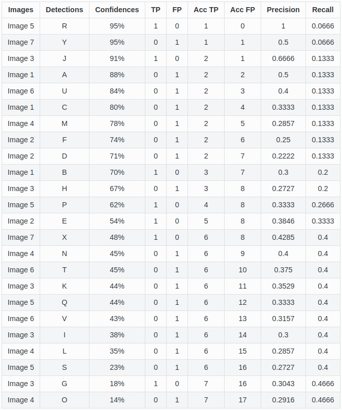
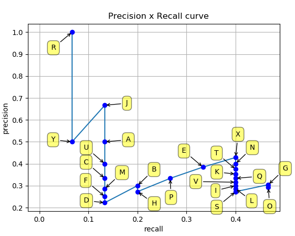
Plotting the precision and recall values we have the following Precision x Recall curve:

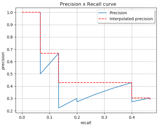
As seen before, the idea of the interpolated average precision is to average the precisions at a set of 11 recall levels (0,0.1,...,1). The interpolated precision values are obtained by taking the maximum precision whose recall value is greater than its current recall value. We can visually obtain those values by looking at the recalls starting from the highest (0.4666) to 0 (looking at the plot from right to left) and, as we decrease the recall, we annotate the precision values that are the highest as shown in the image below:

The Average Precision (AP) is the AUC obtained by the interpolated precision. The intention is to reduce the impact of the wiggles in the Precision x Recall curve. We divide the AUC into 4 areas (A1, A2, A3 and A4) as shown below:

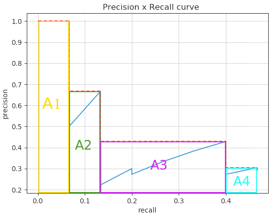
Calculating the total area, we have the AP:

If you want to reproduce these results, see the Sample 2.

How to use this project

This project was created to evaluate your detections in a very easy way. If you want to evaluate your algorithm with the most used object detection metrics, you are in the right place.

Sample_1 and sample_2 are practical examples demonstrating how to access directly the core functions of this project, providing more flexibility on the usage of the metrics. But if you don't want to spend your time understanding our code, see the instructions below to easily evaluate your detections:

Follow the steps below to start evaluating your detections:

1. Create the ground truth files
2. Create your detection files
3. For Pascal VOC metrics, run the command: python pascalvoc.py
   If you want to reproduce the example above, run the command: python pascalvoc.py -t 0.3
4. (Optional) You can use arguments to control the IOU threshold, bounding boxes format, etc.

Create the ground truth files

• Create a separate ground truth text file for each image in the folder groundtruths/.
• In these files each line should be in the format: <class_name> <left> <top> <right> <bottom>.
• E.g. The ground truth bounding boxes of the image "2008_000034.jpg" are represented in the file "2008_000034.txt":

  bottle 6 234 45 362
  person 1 156 103 336
  person 36 111 198 416
  person 91 42 338 500
  

If you prefer, you can also have your bounding boxes in the format: <class_name> <left> <top> <width> <height> (see here * how to use it). In this case, your "2008_000034.txt" would be represented as:

bottle 6 234 39 128
person 1 156 102 180
person 36 111 162 305
person 91 42 247 458

Create your detection files

• Create a separate detection text file for each image in the folder detections/.
• The names of the detection files must match their correspond ground truth (e.g. "detections/2008_000182.txt" represents the detections of the ground truth: "groundtruths/2008_000182.txt").
• In these files each line should be in the following format: <class_name> <confidence> <left> <top> <right> <bottom> (see here * how to use it).
• E.g. "2008_000034.txt":

  bottle 0.14981 80 1 295 500  
  bus 0.12601 36 13 404 316  
  horse 0.12526 430 117 500 307  
  pottedplant 0.14585 212 78 292 118  
  tvmonitor 0.070565 388 89 500 196  
  

Also if you prefer, you could have your bounding boxes in the format: <class_name> <left> <top> <width> <height>.

Optional arguments

Optional arguments:

(*) set -gtformat=xywh and/or -detformat=xywh if format is <left> <top> <width> <height>. Set to -gtformat=xyrb and/or -detformat=xyrb if format is <left> <top> <right> <bottom>.

GitHub