wide-minima-density-hypothesis

Details about the wide minima density hypothesis and metrics to compute width of a minima

This repo presents the wide minima density hypothesis as proposed in the following paper:

Wide-minima Density Hypothesis and the Explore-Exploit Learning Rate Schedule

Key contributions:

Hypothesis about minima density
A SOTA LR schedule that exploits the hypothesis and beats general baseline schedules
Reducing wall clock training time and saving GPU compute hours with our LR schedule (Pretraining BERT-Large in 33% less training steps)
SOTA BLEU score on IWSLT'14 ( DE-EN )

Prerequisite:

CUDA, cudnn
Python 3.6+
PyTorch 1.4.0

Main Results

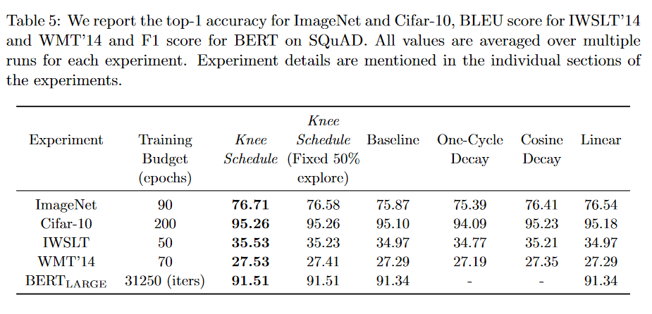
The following table shows comparison of our LR schedule against baseline LR schedules as well as popular LR schedulers available in Pytorch. This comparison is done over the full training budget. For more details about baseline schedules and our LR schedule , please refer to section 5.3 in our paper.

full budget

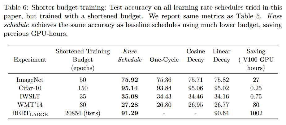
The following table shows comparison of our LR schedule against baseline LR schedules as well as popular LR schedulers available in Pytorch. This comparison is done over a shorter training budget to see how well each schedule generalizes. We demonstrate that our schedule trained with a shorter budget compares with baselines trained on the full budget ( see above table for full budget ). Our hypothesis enables us to save a lot of epochs, thus requiring less GPU utilization. For more details about baseline schedules and our LR schedule , please refer to section 5.3 in our paper.

short budget

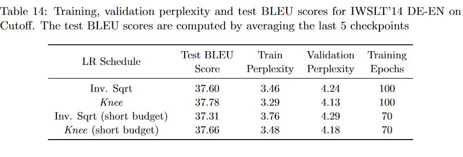
The following table shows comparison of our LR schedule against the inverse square root schedule used by the current SOTA model on IWSLT'14(DE-EN) Cutoff. This comparison is done over the full training budget as well as a shorter training budget. For more details, please refer to section 5.3.6 in our paper.

sota

Hypothesis

We propose a hypothesis that wide/flat minima have a lower density as compared to narrow/sharp minima. We empirically evaluate it on multiple models and datasets. We also show that the initial learning rate phase has a huge role to play in accessing/getting stuck in wider minima and keeping the initial learning rate high for a significant period of time improves the final generalization accuracy on all benchmarks. This initial high learning rate phase is termed as "explore".

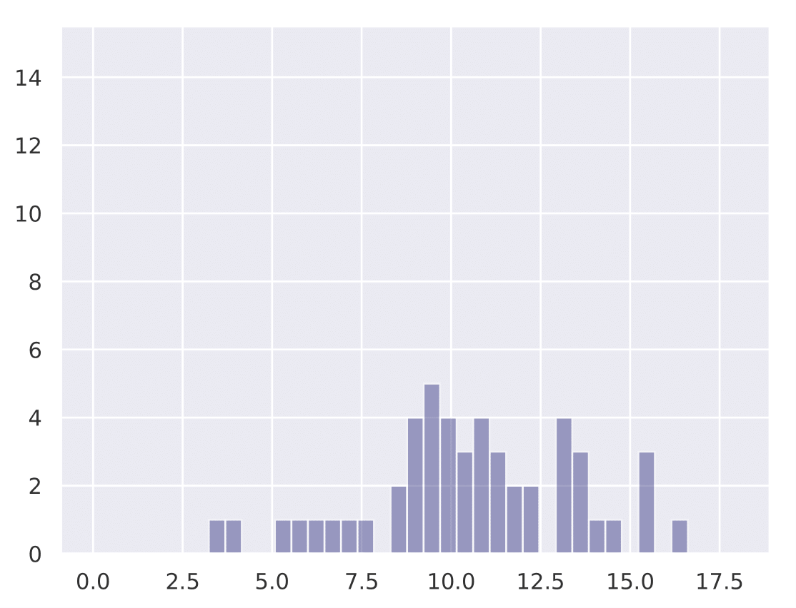
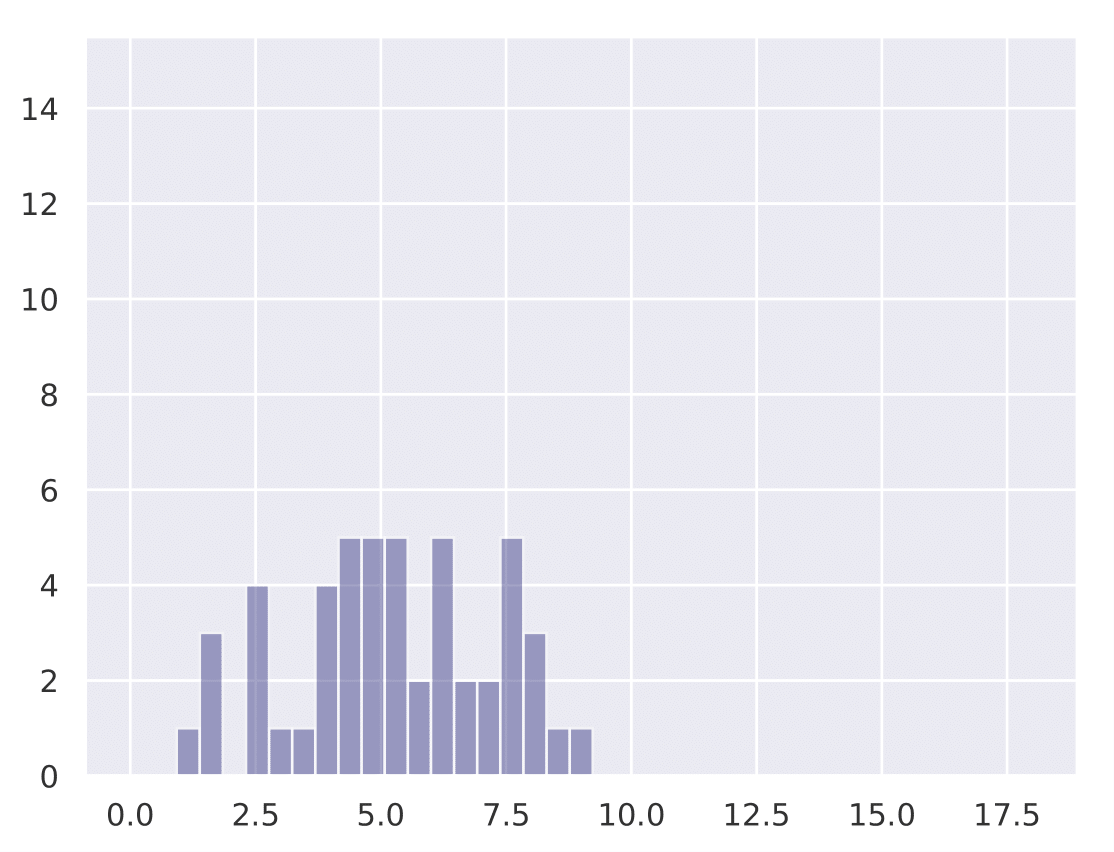
The following histograms show the existence of our hypothesis and how the initial learning rate plays a key role in generalization. We conduct Cifar-10 experiments with Resnet-18 for a total training budget of 200 epochs. We vary the initial phase of explore epochs with 0.1 LR, while dividing the remaining epochs with 0.01 and 0.001 LR respectively. This is done 50 times with different network initializations for each explore setting. We show that as explore epochs is increased, the sharpness of the final minima reduces and generalization on test set improves.

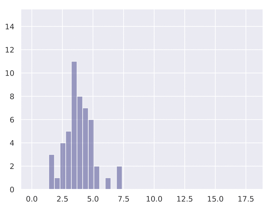
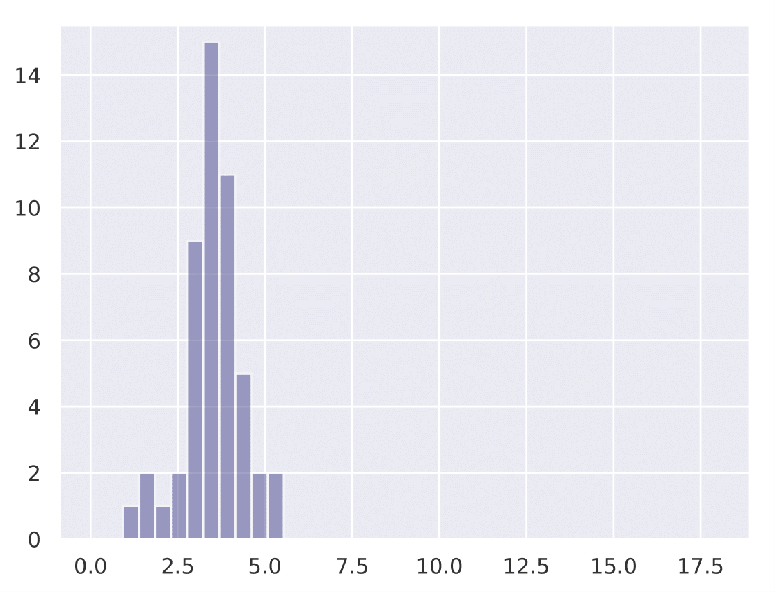
The histograms below shows how sharpness changes as a function of explore. The x axis depicts sharpness and y axis depicts frequency:

0 explore	30 explore	60 explore	100 explore

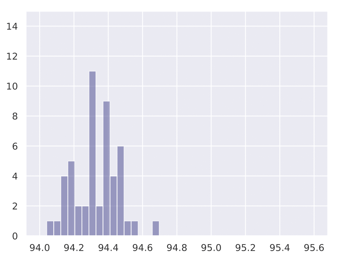
The histograms below shows how final test accuracy changes as a function of explore. The x axis depicts accuracy and y axis depicts frequency:

0 explore	30 explore	60 explore	100 explore

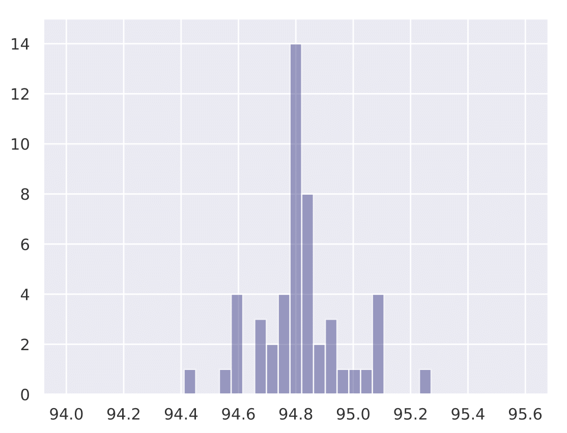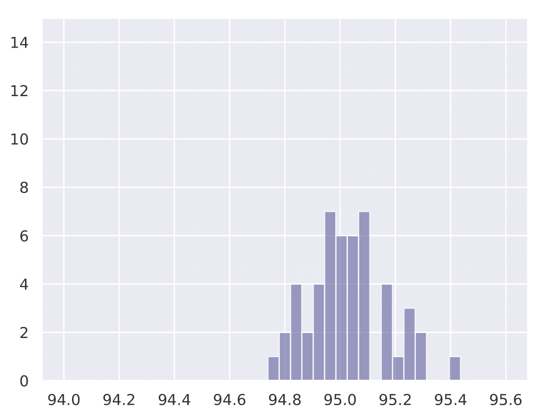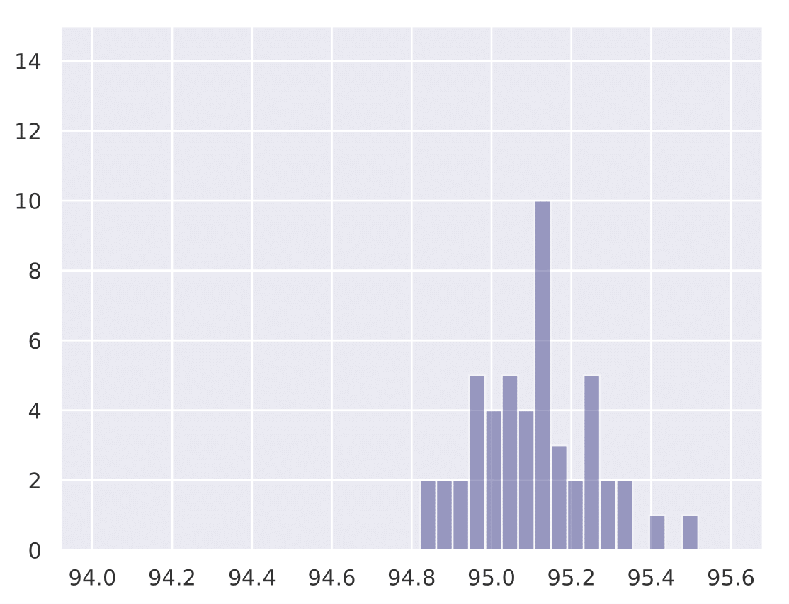Please refer to section 3 in our paper for more details.

PS: We recently wrote another paper where we use our hypothesis to automatically tune the learning rate on various datasets/models. This was accepted at AutoML 2021 workshop conducted alongside ICML 2021. We show boosts in test accuracy as well as reducing training time/steps required for generalization Link

Knee LR Schedule

Based on the density of wide vs narrow minima , we propose the Knee LR schedule that pushes generalization boundaries further by exploiting the nature of the loss landscape. The LR schedule is an explore-exploit based schedule, where the explore phase maintains a high lr for a significant time to access and land into a wide minimum with a good probability. The exploit phase is a simple linear decay scheme, which decays the lr to zero over the exploit phase. The only hyperparameter to tune is the explore epochs/steps. We have shown that 50% of the training budget allocated for explore is good enough for landing in a wider minimum and better generalization, thus removing the need for hyperparameter tuning.

Note that many experiments require warmup, which is done in the initial phase of training for a fixed number of steps and is usually required for Adam based optimizers/ large batch training. It is complementary with the Knee schedule and can be added to it.

To use the Knee Schedule, import the scheduler into your training file:

>>> from knee_lr_schedule import KneeLRScheduler
>>> scheduler = KneeLRScheduler(optimizer, peak_lr, warmup_steps, explore_steps, total_steps)

To use it during training :

>>> model.train()
>>> output = model(inputs)
>>> loss = criterion(output, targets)
>>> loss.backward()
>>> optimizer.step()
>>> scheduler.step()

Details about args:

optimizer: optimizer needed for training the model ( SGD/Adam )
peak_lr: the peak learning required for explore phase to escape narrow minimas
warmup_steps: steps required for warmup( usually needed for adam optimizers/ large batch training) Default value: 0
explore_steps: total steps for explore phase.
total_steps: total training budget steps for training the model

Measuring width of a minima

Keskar et.al 2016 (https://arxiv.org/abs/1609.04836) argue that wider minima generalize much better than sharper minima. The computation method in their work uses the compute expensive LBFGS-B second order method, which is hard to scale. We use a projected gradient ascent based method, which is first order in nature and very easy to implement/use. Here is a simple way you can compute the width of the minima your model finds during training:

>>> from minima_width_compute import ComputeKeskarSharpness
>>> cks = ComputeKeskarSharpness(model_final_ckpt, optimizer, criterion, trainloader, epsilon, lr, max_steps)
>>> width = cks.compute_sharpness()

Details about args:

model_final_ckpt: model loaded with the saved checkpoint after final training step
optimizer : optimizer to use for projected gradient ascent ( SGD, Adam )
criterion : criterion for computing loss (e.g. torch.nn.CrossEntropyLoss)
trainloader : iterator over the training dataset (torch.utils.data.DataLoader)
epsilon : epsilon value determines the local boundary around which minima witdh is computed (Default value : 1e-4)
lr : lr for the optimizer to perform projected gradient ascent ( Default: 0.001)
max_steps : max steps to compute the width (Default: 1000). Setting it too low could lead to the gradient ascent method not converging to an optimal point.

The above default values have been chosen after tuning and observing the loss values of projected gradient ascent on Cifar-10 with ResNet-18 and SGD-Momentum optimizer, as mentioned in our paper. The values may vary for experiments with other optimizers/datasets/models. Please tune them for optimal convergence.

Acknowledgements: We would like to thank Harshay Shah (https://github.com/harshays) for his helpful discussions for computing the width of the minima.

Citation

Please cite our paper in your publications if you use our work:

@article{iyer2020wideminima,
  title={Wide-minima Density Hypothesis and the Explore-Exploit Learning Rate Schedule},
  author={Iyer, Nikhil and Thejas, V and Kwatra, Nipun and Ramjee, Ramachandran and Sivathanu, Muthian},
  journal={arXiv preprint arXiv:2003.03977},
  year={2020}
}