Convex Potential Flows
"Convex Potential Flows: Universal Probability Distributions with Optimal Transport and Convex Optimization" by Chin-Wei Huang, Ricky T. Q. Chen, Christos Tsirigotis, Aaron Courville. In ICLR 2021.
Dependencies:
run pip install -r requirements.txt
Datasets
- For the Cifar 10 / MNIST image modeling experiments: the datasets will be downloaded automatically
using the torchvision package - For the tabular density estimation experiments: download the datasets from
https://github.com/gpapamak/maf - For the VAE experiments, please download the datasets following the instruction in the respective folders of
https://github.com/riannevdberg/sylvester-flows/tree/master/data
Experiments
•• Important ••
Unless otherwise specified, the loss (negative log likelihood) printed during training
is not a measure of the log likelihood; instead it's a "surrogate" loss function explained in the paper:
differentiating this surrogate loss will give us an stochastic estimate of the gradient.
To clarify:
When the model is in the .train() mode, the forward_transform_stochastic function is used to give a stochastic estimate of
the logdet "gradient".
When in .eval() mode, a stochastic estimate of the logdet itself (using Lanczos) will be provided.
The forward_transform_bruteforce function computes the logdet exactly.
As an example, we've used the following context wrapper in train_tabular.py to obtain a likelihood estimate
throughout training:
def eval_ctx(flow, bruteforce=False, debug=False, no_grad=True):
    flow.eval()
    for f in flow.flows[1::2]:
        f.no_bruteforce = not bruteforce
    torch.autograd.set_detect_anomaly(debug)
    with torch.set_grad_enabled(mode=not no_grad):
        yield
    torch.autograd.set_detect_anomaly(False)
    for f in flow.flows[1::2]:
        f.no_bruteforce = True
    flow.train()
Turning flow.no_bruteforce to False will force the flow to calculate logdet exactly in .eval() mode.
Toy 2D experiments
To reproduce the toy experiments, run the following example cmd line
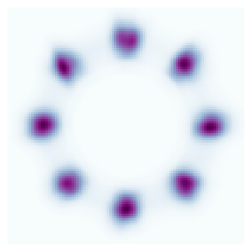
python train_toy.py --dataset=EightGaussian --nblocks=1 --depth=20 --dimh=32
Here's the learned density
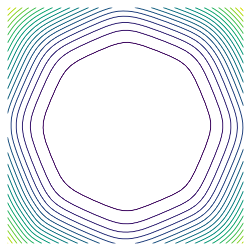
When only one flow layer (--nblocks=1) is used, it will also produce a few interesting plots
for one to analyze the flow, such as the
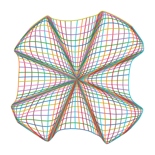
(Convex) potential function
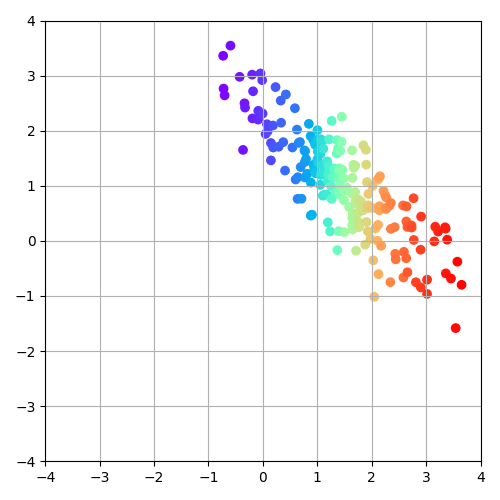
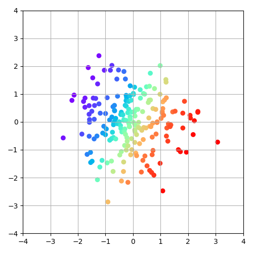
and the corresponding gradient distortion map
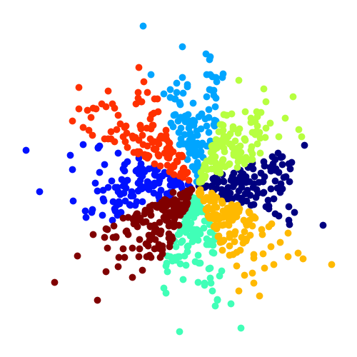
For the 8 gaussian experiment, we've color-coded the samples to visualize the encodings:
Toy image point cloud
We can also set --img_file to learn the "density" of a 2D image as follows:
python train_toy.py --img_file=imgs/github.png --dimh=64 --depth=10
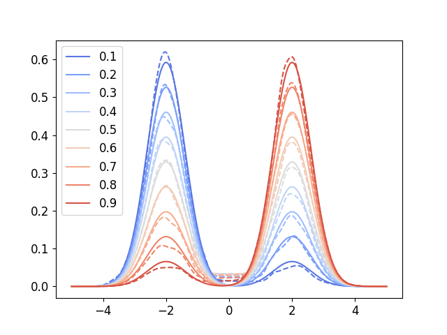
Toy conditional 2D experiments
We've also have a toy conditional experiment to assess the representational power of
the partial input convex neural network (PICNN). The dataset is a 1D mixture of Gaussian
whose weighting coefficient is to be conditioned on (the values in the legend in the following figure).
python train_toy_cond.py
Running the above code will generate the following conditional density curves
OT map learning
To learn the optimal transport map (between Gaussians), run
python train_ot.py
(Modify dimx = 2 in the code for higher dimensional experiments)
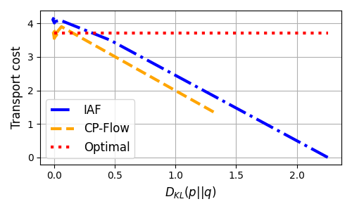
CP-Flow will learn to transform the input Gaussian
into a prior standard Gaussian "monotonically"
This means the transport map is the most efficient one in the OT sense
(in contrast, IAF also learns a transport map with 0 KL, but it has a higher transport cost):
Larger scale experiments
For larger scale experiments reported in the paper, run the following training scripts:
train_img.pyfor the image modeling experimentstrain_tabular.pyfor the tabular data density estimation.
The code is to reproduce the experiments from MAF, based on the
repo https://github.com/gpapamak/maftrain_vae.pyfor improving variational inference (VAE) using flows, which we modified from
Sylvester Flows https://github.com/riannevdberg/sylvester-flows


